Una introducción al descubrimiento causal para marketing y ciencia de datos, presentada en PyData Tallinn 2025.
Autor/a
Carlos Trujillo
Fecha de publicación
1 de febrero de 2025
Introducción al Descubrimiento Causal
En este cuaderno, profundizaremos en cómo descubrir relaciones causales en datos de marketing, un paso crucial para entender el verdadero impacto de los distintos canales en los resultados del negocio. Comenzaremos generando datos sintéticos que imitan escenarios de marketing del mundo real, con variables de confusión y estructuras causales complejas.
A continuación, ajustaremos un modelo Bayesiano de mezcla de marketing usando PyMC-Marketing, verificaremos las direcciones causales entre variables, y realizaremos análisis de mediación para explorar efectos indirectos. Finalmente, usaremos técnicas de descubrimiento de estructura para inferir posibles grafos causales. Al final, tendrás una comprensión sólida de cómo aplicar estas técnicas para revelar conocimientos causales ocultos en tus datos de marketing.
Código
import warningswarnings.filterwarnings("ignore")from pymc_marketing.mmm.transformers import geometric_adstock, michaelis_mentenfrom pymc_marketing.mmm import MMM, GeometricAdstock, MichaelisMentenSaturationfrom pymc_extras.prior import Priorimport networkx as nxfrom graphviz import Digraphimport pydotimport arviz as azimport matplotlib.pyplot as pltimport matplotlib.image as mpimgimport seaborn as snsfrom IPython.display import SVG, displayimport numpy as npimport pandas as pdimport preliz as pzimport pymc as pmfrom PIL import Imagefrom io import BytesIOfrom causallearn.graph.Endpoint import Endpointfrom causallearn.utils.GraphUtils import GraphUtilsfrom causallearn.search.ScoreBased.GES import gesfrom causallearn.search.ConstraintBased.PC import pcaz.style.use("arviz-darkgrid")plt.rcParams["figure.figsize"] = [8, 4]plt.rcParams["figure.dpi"] =100plt.rcParams["axes.labelsize"] =6plt.rcParams["xtick.labelsize"] =6plt.rcParams["ytick.labelsize"] =6plt.rcParams.update({"figure.constrained_layout.use": True})%load_ext autoreload%autoreload 2%config InlineBackend.figure_format ="retina"seed =sum(map(ord, "Estimating effects despite having Confounding Variables"))rng = np.random.default_rng(seed)print(seed)print(rng)
5395
Generator(PCG64)
Caso de negocio
Como empresa probablemente invertimos en diferentes canales para adquirir nuevos clientes. Algunas acciones son más directas, como la publicidad pagada, y otras son más indirectas, como el marketing en medios offline. Como profesionales del marketing y científicos, queremos entender el impacto de cada canal en la variable objetivo (número de nuevos clientes).
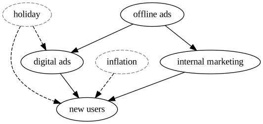
El siguiente DAG muestra una posible estructura causal del problema. Digamos que tenemos las siguientes variables:
x1: publicidad offline, p. ej. TV, radio, prensa, etc.
x2: publicidad digital, p. ej. SEM, SEO, redes sociales, etc.
x3: marketing interno, p. ej. marketing de producto, comunicación interna, etc.
y: nuevos usuarios
Es probable que nuestra publicidad offline no afecte directamente a nuestros nuevos usuarios, pero sí afecta a nuestros anuncios digitales y marketing interno: los usuarios observan un banner de nuestro producto y luego lo buscan en línea, o son referidos por un amigo que finalmente convierte usando su teléfono. De manera independiente, algunos anuncios digitales pueden impactar a usuarios que no habían oído de nosotros antes, y esos podrían convertir directamente.
Además de eso, tenemos algunos factores externos que podrían afectar nuestros nuevos usuarios, p. ej. días festivos, condiciones económicas, etc. Cosas como los días festivos podrían afectar aún más nuestros anuncios digitales, p. ej. más usuarios compran en línea, y estamos invirtiendo más durante esos días también.
Esto crea una estructura causal compleja, donde las variables no son completamente independientes y no es fácil inferir el impacto causal de cada canal en la variable objetivo.
Basándonos en el DAG proporcionado, podemos crear datos sintéticos para probar qué tan bien funciona nuestro modelo cuando tenemos estructuras causales complejas. Usando los mismos datos, podemos probar diferentes composiciones de modelos y ver cómo podríamos mejorar nuestro modelo para descubrir el verdadero impacto causal de cada canal en la variable objetivo.
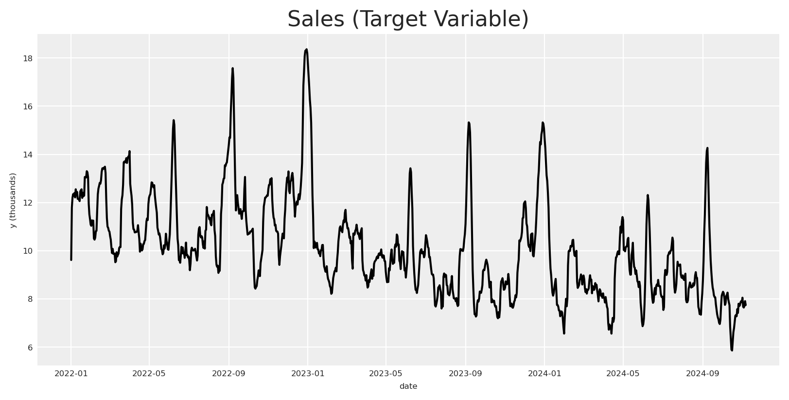
Comenzaremos estableciendo el rango de fechas. Aquí usaremos un rango de fechas del 2022-01-01 al 2024-11-06, lo que significa que tenemos casi 3 años de datos (1041 días).
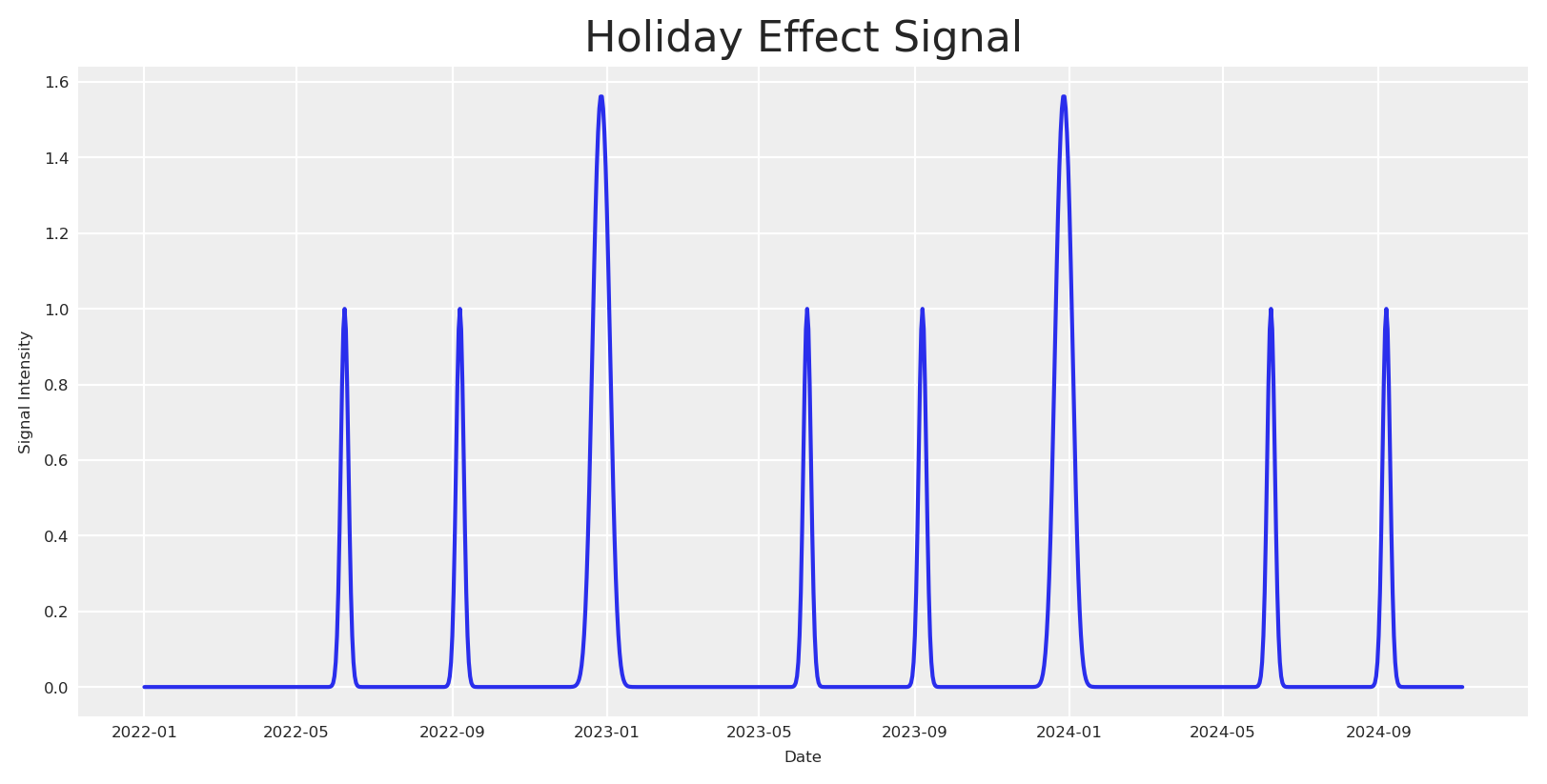
Ciertos días festivos, como la Navidad, pueden tener un impacto significativo en el comportamiento del consumidor antes y después de la fecha específica, generando picos estacionales en ventas. Para capturar estos efectos, introducimos una señal de días festivos basada en distribuciones gaussianas (normales) centradas en fechas festivas específicas.
La función utilizada para modelar el efecto de días festivos se define de la siguiente manera:
Donde: - \Delta t es la diferencia de tiempo (en días) entre la fecha actual y la fecha festiva. - \sigma es la desviación estándar que controla la dispersión del efecto alrededor de la fecha festiva.
Para cada día festivo, calculamos la señal festiva a lo largo del rango de fechas y agregamos una contribución festiva escalando la señal con un coeficiente específico del día festivo. Este enfoque modela los picos estacionales festivos usando funciones gaussianas, que capturan el aumento transitorio en la actividad del mercado alrededor de los días festivos, y su respectiva decadencia a lo largo del tiempo.
Nota: Aquí asumimos una señal distribuida normalmente; sin embargo, la señal podría estar sesgada o no seguir una distribución normal.
Código
holiday_dates = ["24-12", "31-12", "08-06", "07-09"] # List of holidays as month-day stringsstd_devs = [5, 5, 3, 3] # List of standard deviations for each holidayholidays_coefficients = [2, 3, 4, 6]# Initialize the holiday effect arrayholiday_signal = np.zeros(len(date_range))holiday_contributions = np.zeros(len(date_range))# Generate holiday signalsfor holiday, std_dev, holiday_coef inzip( holiday_dates, std_devs, holidays_coefficients, strict=False):# Find all occurrences of the holiday in the date range holiday_occurrences = date_range[date_range.strftime("%d-%m") == holiday]for occurrence in holiday_occurrences:# Calculate the time difference in days time_diff = (date_range - occurrence).days# Generate the Gaussian basis for the holiday _holiday_signal = np.exp(-0.5* (time_diff / std_dev) **2)# Add the holiday signal to the holiday effect holiday_signal += _holiday_signal holiday_contributions += _holiday_signal * holiday_coefdf["holiday_signal"] = holiday_signaldf["holiday_contributions"] = holiday_contributions# Plot the holiday effectfig, ax = plt.subplots()sns.lineplot(x=date_range, y=holiday_signal, ax=ax)ax.set(title="Holiday Effect Signal", xlabel="Date", ylabel="Signal Intensity")plt.show()
Generando inflación
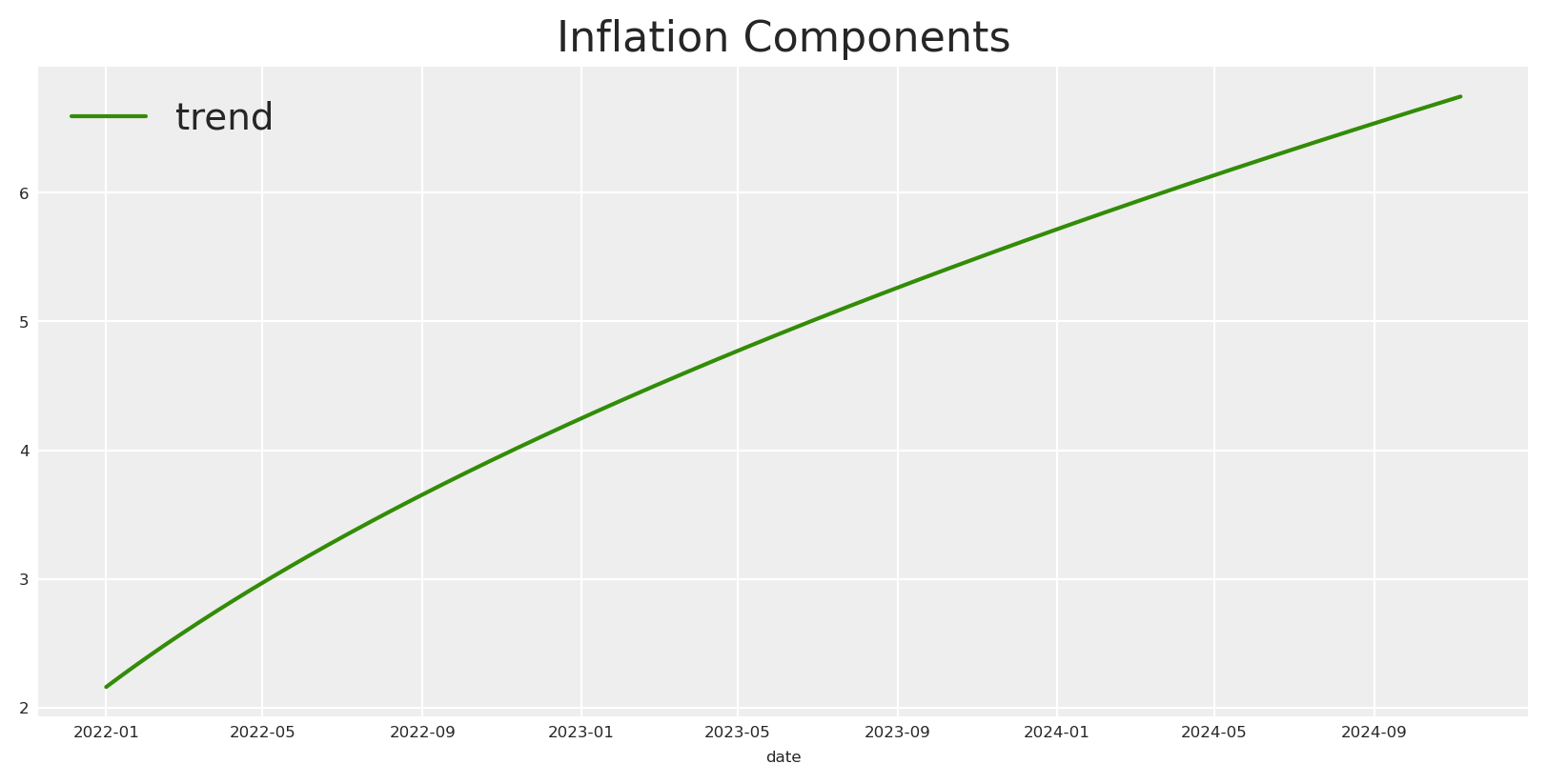
A continuación, generamos los datos de Inflación. Asumimos que la inflación sigue una tendencia de ley de potencias, lo que significa que el crecimiento se acelera con el tiempo en lugar de permanecer constante. Esto se puede definir matemáticamente como:
Donde: - t: El índice temporal, representando los días desde el inicio del rango de fechas. - baseline: Una constante sumada a t para desplazar el punto de inicio de la tendencia. Este valor afecta el nivel inicial de crecimiento del mercado. El valor inicial de la función será (baseline)^{exponent} - 1, no 0. - exponent: La potencia a la que se eleva el índice temporal, determinando la tasa a la que la tendencia se acelera con el tiempo.
En esta sección, simulamos tres canales de marketing, x1, x2 y x3, que representan diferentes canales publicitarios (p. ej., Marketing Interno, Marketing Social, Marketing Offline). El comportamiento de cada canal está influenciado por la variabilidad aleatoria y los efectos de confusión de los días festivos estacionales. Así es como modelamos cada canal matemáticamente:
Canal x1: Como mencionamos antes, generamos x1 que es afectado por la señal de días festivos, podríamos definirlo como:
I_{x1_t} = S_{x1_t} + e_{x1}
Canal x2: Por otro lado, generamos x2 que es afectado por la señal de días festivos y la influencia de x1. Podríamos definirlo como:
Estas ecuaciones nos permiten capturar la dinámica compleja que influye en cada canal de marketing: - Los Efectos de Días Festivos aumentan la actividad del canal alrededor de fechas específicas, simulando picos estacionales. - Las Influencias entre Canales introducen interdependencias, modelando cómo el éxito de un canal puede amplificar el de otro.
Nota: Aquí estamos asumiendo un impacto aditivo para las interacciones entre canales.
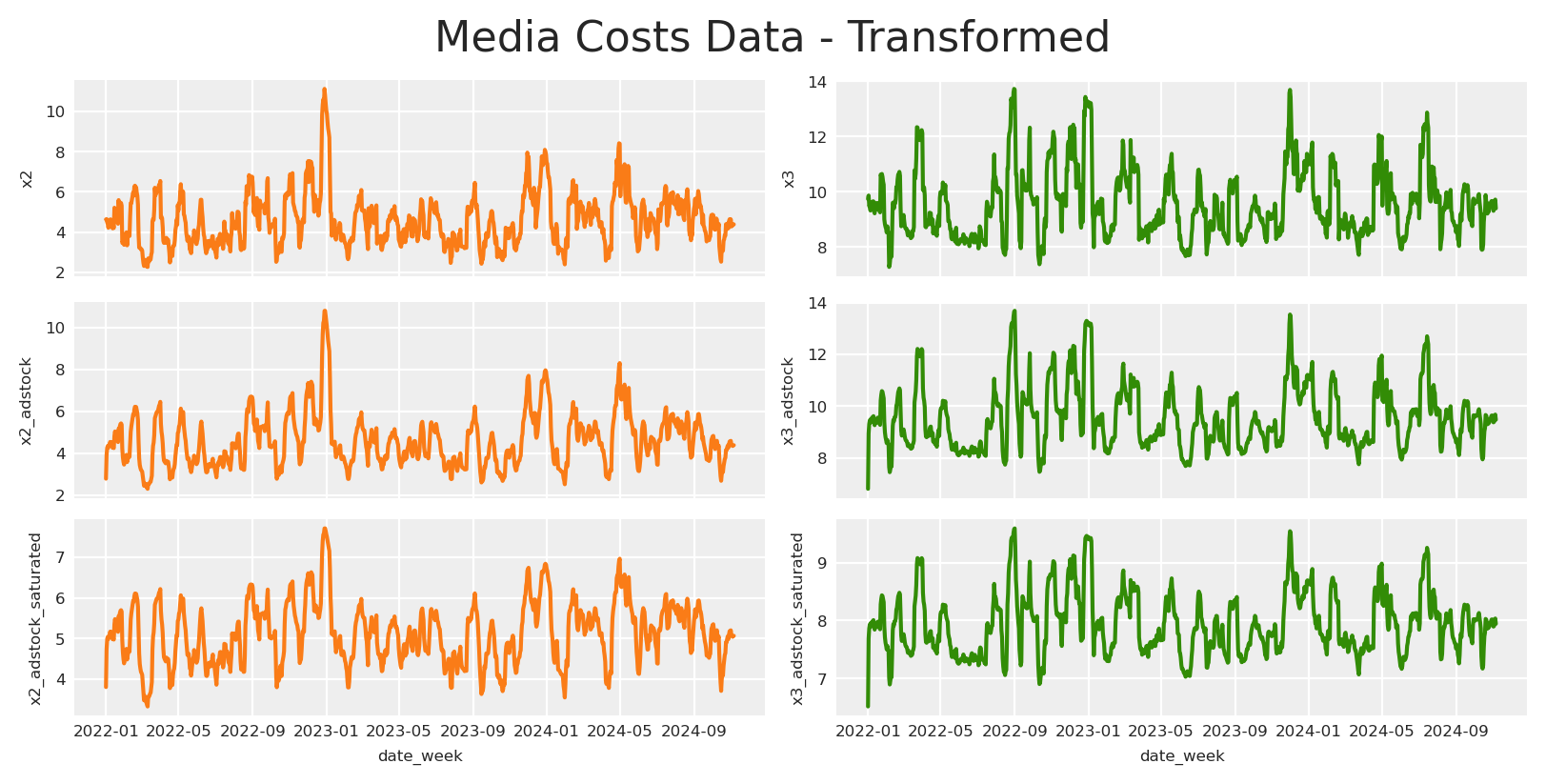
Asumiremos que todas las actividades de marketing sufren las mismas transformaciones de Adstock y Saturación. Esto significa que cada canal tendrá parámetros individuales para las transformaciones seleccionadas, en este caso adstock geométrico y Michaelis-Menten.
Donde: - Intercepto: Un nivel base de ventas, establecido en 1.5, representando el nivel base de ventas en ausencia de otros efectos. - Inflación: Representa la inflación subyacente del mercado, con un coeficiente negativo implícito de 1, añadiendo una influencia descendente constante. - Contribuciones de Días Festivos: Añade picos de ventas alrededor de los períodos festivos, capturando el aumento estacional en la demanda del consumidor. - m(Impressions_{x3_t}) y m(Impressions_{x2_t}): Representan los valores de adstock saturado para los canales de marketing x3 y x2. - Ruido \epsilon: Un término de error aleatorio pequeño, extraído de una distribución normal con media 0 y desviación estándar 0.08, para dar cuenta de la variabilidad inexplicada en las ventas.
Podemos escalar el conjunto de datos completo y finalmente tendremos algo muy similar a la realidad.
Código
# scale df by abs max per columndf["date"] = pd.to_datetime(df["date_week"])scaled_df = df.copy()for col in scaled_df.columns:if col !='date'and col !='date_week': scaled_df[col] = scaled_df[col] / scaled_df[col].abs().max()scaled_df[["date", "x1", "x2", "x3", "y"]].head()
date
x1
x2
x3
y
0
2022-01-01
0.311103
0.416608
0.709209
0.523628
1
2022-01-02
0.346200
0.417910
0.718519
0.641921
2
2022-01-03
0.310798
0.404066
0.690251
0.664626
3
2022-01-04
0.301643
0.395861
0.693495
0.672532
4
2022-01-05
0.248688
0.379114
0.679055
0.668596
Enfoque inicial
Si tenemos un conjunto de datos como el que acabamos de crear, podemos intentar ajustar un modelo con lo siguiente para encontrar el impacto causal de cada canal en la variable objetivo. Para el ejemplo, usaremos un modelo simple de PyMC-Marketing para este propósito.
Veamos qué sucede si ajustamos un modelo con todo lo que tenemos sin ningún conocimiento de la estructura causal.
Como era de esperar, el modelo no logra reflejar con precisión las contribuciones reales, resultando en estimaciones que se desvían significativamente de los valores reales. ¿Cómo puede ocurrir esto, y por qué está sucediendo?
La explicación es sencilla: al descuidar cualquier estructura causal, inadvertidamente imponemos una sobre los datos. El problema radica en nuestra suposición del marco causal más simple, que rara vez se alinea con la complejidad del mundo real.
¿Qué tipo de estructura causal estamos asumiendo implícitamente cuando ajustamos el modelo?
Código
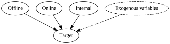
# Initialize a directed graphnaive_causal_mmm_graph = Digraph()# Add nodesnaive_causal_mmm_graph.node("X1", "Offline")naive_causal_mmm_graph.node("X2", "Online")naive_causal_mmm_graph.node("X3", "Internal")naive_causal_mmm_graph.node("E", "Exogenous variables", style="dashed")naive_causal_mmm_graph.node("T", "Target")naive_causal_mmm_graph.edge("E", "T", style="dashed")naive_causal_mmm_graph.edge("X1", "T")naive_causal_mmm_graph.edge("X2", "T")naive_causal_mmm_graph.edge("X3", "T")# Render the graph to SVG and display it inlinesvg_str = naive_causal_mmm_graph.pipe(format="svg")display(SVG(svg_str))
El DAG anterior representa la estructura causal que estamos asumiendo implícitamente cuando ajustamos el modelo. Aquí todas las variables son independientes entre sí, y esas impactan directamente la variable objetivo.
Durante el desarrollo del modelo, establecimos una estructura y flujo específicos para nuestros datos. Concluimos que los impactos de nuestros canales operan de manera independiente entre sí. Además, determinamos que si algún componente de nuestro ecosistema falta, su influencia será capturada por el término base debido a esta ecuación. Como puedes ver, incluso adoptando este modelo básico, estamos haciendo suposiciones significativas.
Por un lado, estás asumiendo que el impacto no es lineal al aplicar estas transformaciones, y estás sugiriendo que el impacto es positivo y que puede haber un retraso máximo de un cierto número de días.
Incluso has definido la dirección de tus relaciones. Al definir estas relaciones y asumir que no hay conexiones causales directas entre nuestras variables, podemos concluir que, si la naturaleza de su relación está representada con precisión por la ecuación proporcionada, entonces al controlar los canales relevantes, podríamos descubrir sus verdaderos efectos.
Esto nos lleva a qué DAG causal asumimos como correcto, basándonos en nuestras suposiciones previas. Si reconoces este proceso, ¡felicidades! Has creado un modelo generativo o Modelo Causal Estructural, con una Ecuación Causal Estructural, usando PyMC-Marketing.
Sin embargo, este DAG Causal no representa el verdadero DAG Causal. Dado que nuestro modelo de PyMC es estructural y causal, debemos preguntar: ¿Qué sucede si creo un modelo con una estructura causal diferente a la real?
La respuesta es lo que observamos arriba, el modelo no podrá recuperar la verdadera estructura causal.
Aprendiendo sobre modelos generativos
Los modelos generativos son marcos que describen cómo podrían producirse los datos en el mundo real. Definen un proceso al establecer distribuciones de probabilidad para cada componente, simulando la creación de datos a partir de variables aleatorias subyacentes. Este enfoque captura la incertidumbre y la variabilidad, proporcionando un panorama completo del mecanismo de generación de datos.
En PyMC, este concepto está en el núcleo de cada modelo. PyMC te permite definir explícitamente priors, verosimilitudes y la estructura de tu proceso de generación de datos. Incluso los modelos simples construidos en PyMC llevan una suposición generativa inherente, haciéndolos flexibles y robustos para representar cómo los datos podrían surgir naturalmente.
Esto significa que cada posible grafo con N número de variables puede ser un modelo específico. ¿Cuántos modelos podríamos especificar si tenemos 5 variables para un objetivo?
Código
import mathfrom functools import lru_cache@lru_cache(maxsize=None)def dag_with_exactly_s_sources(n: int, s: int) ->int:""" Count DAGs with exactly s source nodes. Uses formula: S(n,s) = C(n,s) * sum[(-1)^j * C(n-s,j) * 2^((m-j)(m-j-1)/2) * (2^(m-j)-1)^s] where m=n-s and j=0..m. When n=s, S(n,n)=1. Parameters ---------- n : int Total number of labeled nodes s : int Number of source nodes Returns ------- int Number of possible DAGs """if n == s:return1 total =0 m = n - sfor j inrange(m +1): term = ( (-1) ** j* math.comb(m, j)*2** (((m - j) * (m - j -1)) //2)* (2** (m - j) -1) ** s ) total += termreturn math.comb(n, s) * totaldef count_valid_final_graphs_with_parents(num_regressors: int, num_parents: int) ->int:"""Count valid final graphs with parent node restrictions. The counting process has two main steps: 1. Build a DAG among regressors where parents have no incoming edges: - For non-parents (Q = num_regressors - num_parents), count DAGs with given sinks - Parents can only have edges to non-parents (Q options each) - Non-sink parents must have ≥1 outgoing edge (2^Q - 1 ways) - Sink parents have no edges (1 way) 2. Add edges from regressors to target: - Sink regressors must connect to target - Non-sink regressors optionally connect - Yields factor 2^(num_regressors - total_sinks) The total count formula is: sum_{s_p=0}^P sum_{s_q=1}^Q [binom(P,s_p) * (2^Q-1)^(P-s_p) * (DAGs_Q_s_q) * 2^((P+Q)-(s_p+s_q))] where P = num_parents, Q = num_regressors - num_parents When Q = 0 (all regressors are parents), the final graph is unique. Parameters ---------- num_regressors : int Total number of regressor nodes in the graph num_parents : int Number of designated parent nodes that cannot have incoming edges Returns ------- int Total count of valid final graph configurations """ P = num_parents Q = num_regressors - num_parents # non-parentsif Q <0:raiseValueError("num_parents cannot exceed num_regressors")# Case where all regressors are parents: no DAG edges are allowed;# every node is isolated (and hence a sink),# so the regressor-to-target assignment is forced.if Q ==0:return1 total =0# s_p: number of parents that end up as sinks# (i.e. with no outgoing edge to any non-parent)for s_p inrange(P +1):# For each parent:# - If not a sink: choose at least one outgoing edge# among Q non-parents: (2^Q - 1) ways.# - If a sink: only 1 way (choose no outgoing edge). parent_config = math.comb(P, s_p) * ((2**Q -1) ** (P - s_p))# s_q: number of sinks among non-parents in the DAG on Q nodes.# Note: Every DAG on at least one node has at least one sink.for s_q inrange(1, Q +1): nonparent_count = dag_with_exactly_s_sources(Q, s_q)# Total sinks in the regressor# DAG is s_p (from parents) plus s_q (from non-parents) total_sinks = s_p + s_q# For each regressor that is not a sink,# the regressor-to-target edge is optional.# Thus, a factor of 2^( (P+Q) - total_sinks ). assignment_factor =2** ((P + Q) - total_sinks) total += parent_config * nonparent_count * assignment_factorreturn totalpossible_dags = count_valid_final_graphs_with_parents(num_regressors=5, num_parents=2)print(f"Number of possible DAGs with two parents (Graphical/Generative Model): {possible_dags:,}")possible_dags = count_valid_final_graphs_with_parents(num_regressors=5, num_parents=1)print(f"Number of possible DAGs with one parent (Graphical/Generative Model): {possible_dags:,}")
Number of possible DAGs with two parents (Graphical/Generative Model): 12,375
Number of possible DAGs with one parent (Graphical/Generative Model): 52,855
El número de modelos posibles que podemos generar con dos de cinco variables como padres es de alrededor de 12.000, mientras que tener solo un padre aumenta ese número a aproximadamente 52.000. Curiosamente, eliminar un solo nodo padre triplica los modelos potenciales que podemos crear, multiplicando efectivamente el número de escenarios posibles.
Esto arroja luz sobre los desafíos que plantean los modelos grandes:
a) A medida que aumenta el número de variables, el crecimiento exponencial en relaciones potenciales se vuelve abrumador, dificultando identificar nuestra situación real.
b) Con más variables, la probabilidad de controlar erróneamente por las variables equivocadas también aumenta.
Este último punto se alinea con nuestra observación anterior: si controlamos por variables inapropiadas, el modelo no logra recuperar la verdadera estructura causal.
Entonces, ¿por qué es problemático controlar por ciertas variables? Cada variable debería agregar más poder explicativo, ¿no? Empecemos a aprender sobre estructuras para entenderlo.
Aprendiendo sobre estructuras causales
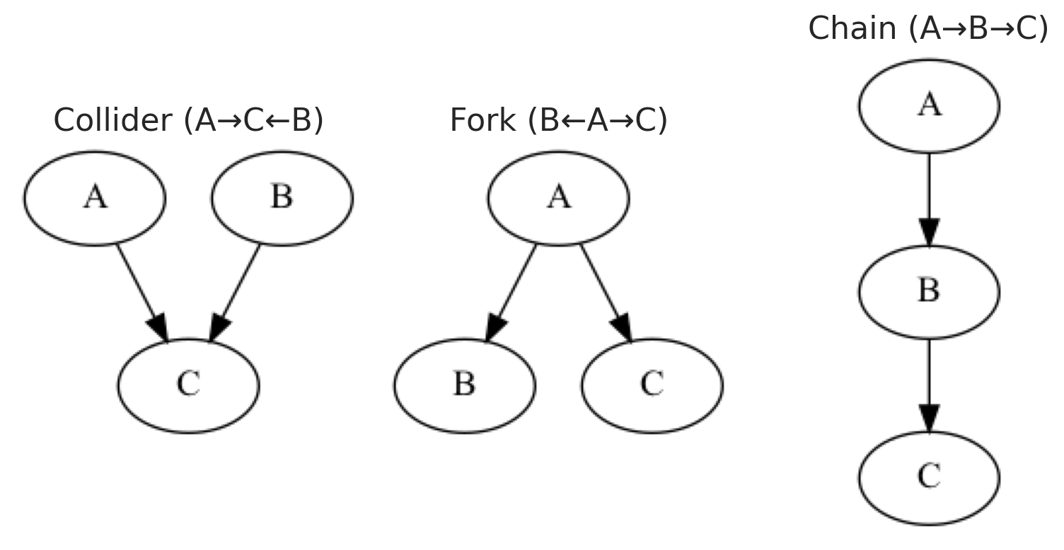
Bifurcaciones: Una bifurcación es una estructura causal donde una sola variable actúa como causa común para dos o más variables. Esta causa común transmite su influencia a todos sus descendientes directos. La existencia de una bifurcación crea confusión, haciendo que la relación entre las variables descendientes parezca estar relacionada. Controlar por la causa común puede bloquear efectivamente las vías de retroceso creadas por esta estructura.
Cadenas: Una cadena representa una vía causal secuencial donde una variable influye en otra, que a su vez afecta a una tercera. Esta estructura destaca el proceso de mediación a través del cual se transmiten los efectos causales. La variable intermedia actúa como mediadora, transmitiendo la influencia desde la causa inicial hasta el resultado final. Analizar cadenas ayuda a distinguir entre efectos directos e indirectos en un sistema causal. Controlar por el mediador de manera inapropiada puede bloquear partes del efecto causal que son de interés.
Colisionadores: Un colisionador es una variable que es el efecto común de dos o más factores causales. Se sitúa en la convergencia de diferentes vías causales y puede introducir asociaciones espurias cuando se condiciona sobre él. Controlar por un colisionador puede abrir inadvertidamente vías no causales de retroceso (backdoor), llevando a estimaciones sesgadas. Este fenómeno, conocido como sesgo de colisión, distorsiona las relaciones verdaderas entre las variables causales. Evitar condicionar sobre colisionadores es crucial para mantener la validez de los modelos causales.
Las estructuras causales juegan un papel crucial en diversos métodos de inferencia causal, sirviendo como base para su funcionamiento. Por ejemplo, las estructuras de cadena son clave para métodos como las variables instrumentales (VI). En el análisis de VI, esta estructura de cadena entra en juego al introducir un instrumento: una variable que afecta la exposición pero no afecta directamente el resultado, excepto a través de esa exposición. Este enfoque ayuda a romper la vía de confusión, permitiéndonos aislar la variación exógena en el tratamiento.
Como resultado, permite una estimación consistente de los efectos causales, incluso cuando encontramos endogeneidad. Por lo tanto, comprender las estructuras de cadena es esencial, ya que no solo respalda la lógica detrás de los métodos de VI, sino que también subraya la importancia de identificar instrumentos válidos.
Si te interesa especialmente aprender más sobre VI, te recomiendo consultar una publicación de Anton Bugaev o dirigirte al quinto piso si estás en Bolt.
En última instancia, cada una de estas estructuras causales exhibe diferentes comportamientos observacionales. Esto significa que, basándonos en los datos observacionales, podemos deducir qué estructura está presente y, en consecuencia, determinar cuál es el conjunto correcto de variables a controlar.
Una cosa para entender qué controlar es encontrar los nodos padres para evitar controlar por mediadores. Podríamos identificar esto comprendiendo las dependencias condicionales.
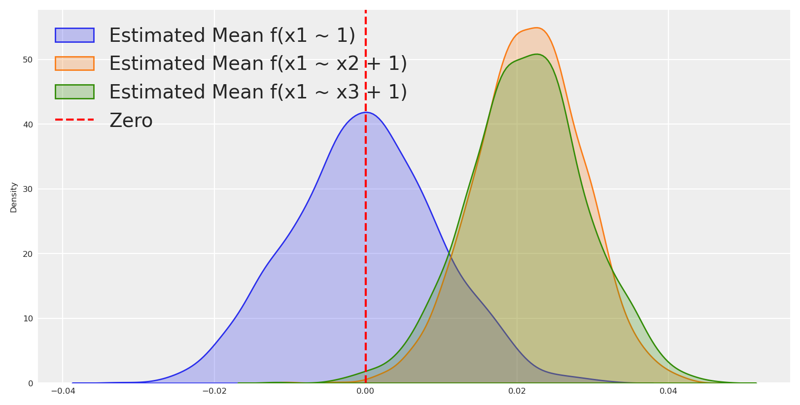
Verifiquemos las independencias condicionales
La independencia condicional es un concepto central en la teoría de probabilidad y la estadística donde dos variables son independientes entre sí una vez que una tercera variable se mantiene constante. Esto significa que, dado el valor de la variable de condicionamiento, las dos variables no proporcionan información adicional la una sobre la otra. En el descubrimiento causal, las independencias condicionales son cruciales porque revelan la estructura subyacente de las relaciones causales en un modelo o un grafo acíclico dirigido (DAG). Al identificar estas independencias, podemos determinar cómo están relacionadas las variables entre sí, o no.
Los modelos de regresión Bayesiana nos permiten estimar la expectativa condicional de un resultado dado un conjunto de predictores, descubriendo efectivamente las probabilidades condicionales subyacentes. En una regresión lineal Bayesiana, por ejemplo, estimamos E(Y \mid X) = \beta_0 + \beta_1X_1 + \ldots + \beta_kX_k, que representa el resultado promedio Y cuando los predictores X_1, \dots, X_k se mantienen en valores específicos.
Definamos una función para construir y muestrear un modelo lineal a partir de una fórmula.
Código
def build_and_sample_model(data: pd.DataFrame, formula: str):""" Build and sample a linear model from a formula. """# Parse the formula to get target and channels target, channels = formula.split('~') target = target.strip() channels = [ch.strip() for ch in channels.split('+') if ch.strip() !="1"]# Define coordinates coordinates = {"date": data.date.unique()}if channels: # If there are regressors, include them in coordinates coordinates["channel"] = channels# Filter the dataset based on the formulawith pm.Model(coords=coordinates) as linear_model:# Load Data in Model target_data = pm.Data("target", data[target].values, dims="date")# Constant or intercept intercept = pm.Gamma("intercept", mu=3, sigma=2) mu_var =0if channels: # If there are regressors, include them regressors = pm.Data("regressors", data[channels].values, dims=("date", "channel")) gamma = pm.Normal("gamma", mu=3, sigma=2, dims="channel") mu_var += (regressors * gamma).sum(axis=-1) + interceptelse: mu_var += intercept# Likelihood pm.Normal("likelihood", mu=mu_var, sigma=pm.Gamma("sigma", mu=2, sigma=3), observed=target_data, dims="date")# Sample idata = pm.sample_prior_predictive(random_seed=42) idata.extend( pm.sample(tune=1000, draws=500, chains=4, random_seed=42, target_accept=0.9, nuts_sampler="numpyro", progressbar=False) ) pm.compute_log_likelihood(idata, progressbar=False) idata.extend( pm.sample_posterior_predictive(idata, random_seed=42) )return (idata, linear_model)
Ahora, construyamos y muestreemos los modelos para cada variable.
En un sistema causal donde la dirección verdadera es x_1 a x_2, la distribución conjunta se factoriza como
P(x_1, x_2) = P(x_1) \, P(x_2 \mid x_1),
donde x_1 es exógeno e independiente de cualquier efecto. Esta estructura refleja que la distribución de x_1 permanece sin cambios independientemente de la variable aguas abajo x_2.
Al regresar x_2 sobre x_1, el modelo aprovecha la dirección causal, y la distribución condicional P(x_2 \mid do(x_1)) está más concentrada que la marginal P(x_2). Esto resulta en residuos centrados alrededor de cero, indicando que la mayor parte de la variabilidad en x_2 es explicada por x_1.
En contraste, invertir la regresión modelando x_1 como función de x_2 interrumpe el orden causal. La distribución condicional P(x_1 \mid do(x2)) se desvía de la marginal verdadera P(x_1), ya que intenta capturar la causa a partir de su efecto, lo cual no está respaldado por la estructura causal.
El sesgo en la regresión inversa surge porque condicionar sobre x_2 introduce variabilidad del ruido inherente en x_2. Esta mala atribución confunde la variabilidad independiente de x_1 con la inducida por x_2, llevando a residuos que se desvían sistemáticamente del cero. Respecto al modelo nulo, los residuos están más lejos de cero.
Esta discrepancia subraya la importancia de preservar la dirección causal correcta para evitar sesgo, ya que invertir la regresión viola la condición de Markov causal.
Usando esta lógica, podemos identificar no solo variables independientes sino también los padres candidatos para cada variable basándonos en cómo se desvían del modelo nulo.
Código
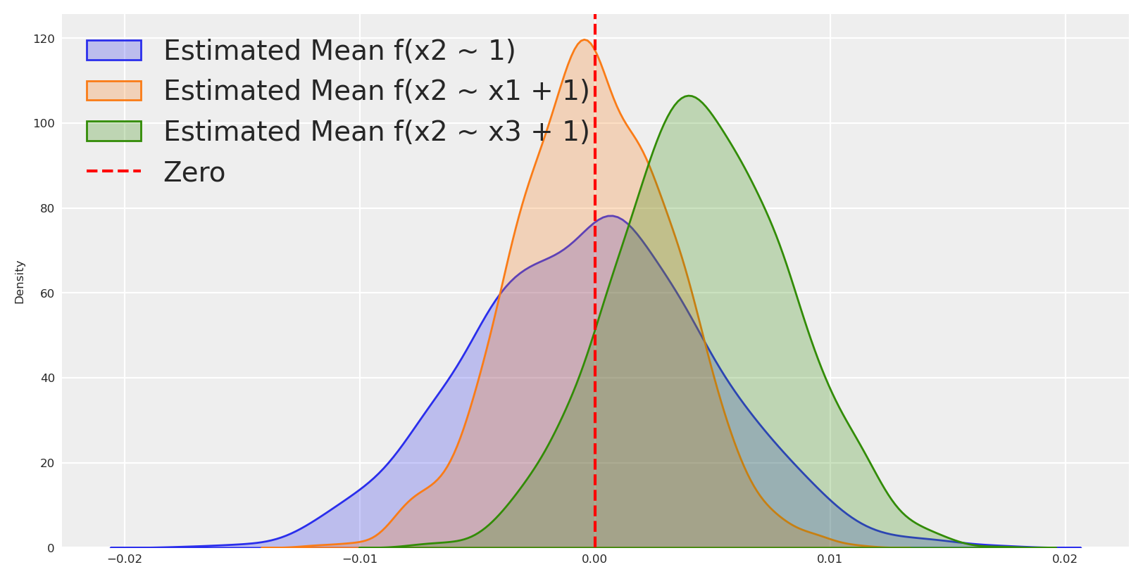
idata1, model1 = build_and_sample_model(scaled_df,"x2 ~ 1")idata2, model2 = build_and_sample_model(scaled_df,"x2 ~ x1 + 1")idata3, model3 = build_and_sample_model(scaled_df,"x2 ~ x3 + 1")idata4, model4 = build_and_sample_model(scaled_df,"x2 ~ x1 + x3 + 1")_real_mean = scaled_df["x2"].mean()_estimated_mean1 = idata1.posterior_predictive.likelihood.mean(dim=["date"]).values.flatten()_estimated_mean2 = idata2.posterior_predictive.likelihood.mean(dim=["date"]).values.flatten()_estimated_mean3 = idata3.posterior_predictive.likelihood.mean(dim=["date"]).values.flatten()#plot distribution of means and real mean as vertical linesns.kdeplot(_estimated_mean1 - _real_mean, label='Estimated Mean f(x2 ~ 1)', fill=True)sns.kdeplot(_estimated_mean2 - _real_mean, label='Estimated Mean f(x2 ~ x1 + 1)', fill=True)sns.kdeplot(_estimated_mean3 - _real_mean, label='Estimated Mean f(x2 ~ x3 + 1)', fill=True)plt.axvline(0, color='red', linestyle='--', label='Zero')plt.legend()plt.show()
Sampling: [gamma, intercept, likelihood, sigma]
The rhat statistic is larger than 1.01 for some parameters. This indicates problems during sampling. See https://arxiv.org/abs/1903.08008 for details
Sampling: [likelihood]
Aquí podemos ver que los residuos están centrados alrededor de cero cuando regresamos la probabilidad marginal de x_2, pero están más cerca de cero con una distribución de probabilidad más estrecha que el modelo nulo cuando regresamos x_2 sobre x_1. Esta es una buena señal de que x_1 es un padre de x_2.
Podemos repetir este proceso para todas las variables en nuestro conjunto de datos para empezar a identificar los padres de cada variable, y así identificar secciones del grafo causal verdadero.
Implementemos esto en código.
Identificando Candidatos a Padres
Para identificar sistemáticamente las variables padres potenciales en nuestro grafo causal, crearemos una clase que evalúe diferentes modelos de regresión y compare sus distribuciones de residuos. Este enfoque aprovecha el principio de que cuando modelamos correctamente la dirección causal, los residuos deberían estar más concentrados alrededor de cero en comparación con modelos mal especificados.
Advertencia
Aunque este enfoque proporciona una buena señal inicial para las relaciones causales, tiene limitaciones. El método asume relaciones lineales, no tiene en cuenta los factores de confusión ocultos, y puede tener dificultades con estructuras causales complejas. Los resultados deben considerarse como evidencia preliminar más que como prueba definitiva de relaciones causales.
La clase ParentCandidateIdentifier a continuación hará lo siguiente: 1. Ejecutar un modelo base solo con un intercepto 2. Ejecutar modelos con cada variable potencial padre 3. Comparar cuánta masa de probabilidad se concentra cerca de cero en las distribuciones de residuos 4. Identificar variables que mejoran el ajuste del modelo como candidatos a padres potenciales
Código
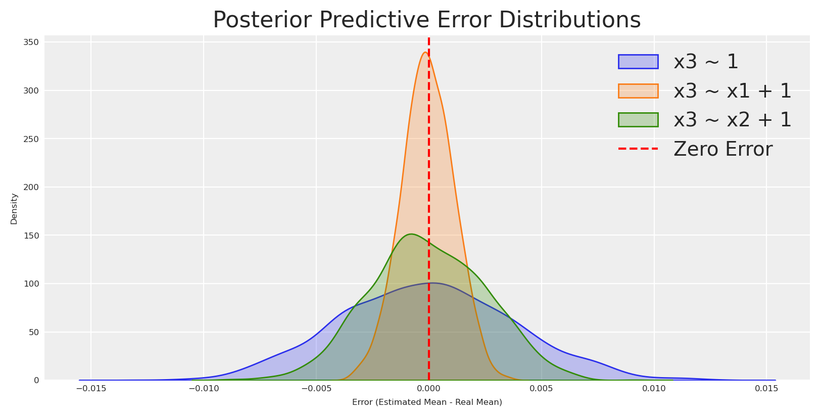
class ParentCandidateIdentifier:def__init__(self, data: pd.DataFrame, node: str, possible_parents: list, epsilon: float=0.005):""" Parameters: data: DataFrame containing your data. node: The target variable for which to identify candidate parents. possible_parents: A list of potential parent variable names. epsilon: Threshold to define "mass around zero" (default 0.05). """self.data = dataself.node = nodeself.possible_parents = possible_parentsself.epsilon = epsilonself.runs = {}self.results =Nonedef build_and_sample_model(self, formula: str):"""Wrapper for the sampling function."""return build_and_sample_model(self.data, formula)def compute_mass_around_zero(self, idata, real_mean):""" Compute the fraction of posterior predictive likelihood samples (averaged over dates) within epsilon of the real mean. """ estimated_mean = idata.posterior_predictive.likelihood.mean(dim=["date"]).values.flatten() distribution = estimated_mean - real_mean mass = np.mean(np.abs(distribution) <self.epsilon)return mass, distributiondef run_all_models(self):""" Run the intercept-only model and each individual parent's model, storing the sampling results, mass, and error distributions. """ real_mean =self.data[self.node].mean() runs = {}# Intercept-only model: P(node) formula_intercept =f"{self.node} ~ 1" idata_int, _ =self.build_and_sample_model(formula_intercept) mass_int, dist_int =self.compute_mass_around_zero(idata_int, real_mean) runs["intercept_only"] = {"formula": formula_intercept,"idata": idata_int,"mass": mass_int,"distribution": dist_int }# Individual candidate parent models: P(node|parent)for parent inself.possible_parents: formula_parent =f"{self.node} ~ {parent} + 1" idata_parent, _ =self.build_and_sample_model(formula_parent) mass_parent, dist_parent =self.compute_mass_around_zero(idata_parent, real_mean) runs[f"parent_{parent}"] = {"formula": formula_parent,"idata": idata_parent,"mass": mass_parent,"distribution": dist_parent }self.runs = runsreturn runsdef identify_candidate_parents(self):""" Runs all models (if not already run), compares the mass around zero, and returns a decision: if the intercept-only model is best, the target is independent; otherwise, return the candidate parent with the highest mass. """ifnotself.runs:self.run_all_models() best_key, best_info =max(self.runs.items(), key=lambda x: x[1]["mass"])if best_key =="intercept_only": decision ="independent" candidate_parents = []else: decision ="dependent" candidate_parents = [best_key.split("_", 1)[1]]self.results = {"results": self.runs,"best_model": {best_key: best_info},"decision": decision,"candidate_parents": candidate_parents }returnself.resultsdef plot_distributions(self):""" Plot the error distributions from the stored runs using Seaborn. """ifnotself.runs:self.run_all_models()for key, run inself.runs.items(): sns.kdeplot(run["distribution"], label=run["formula"], fill=True) plt.axvline(0, color='red', linestyle='--', label='Zero Error') plt.xlabel("Error (Estimated Mean - Real Mean)") plt.ylabel("Density") plt.title("Posterior Predictive Error Distributions") plt.legend() plt.show()
Ahora podemos identificar los candidatos a padres para cada variable.
Sampling: [gamma, intercept, likelihood, sigma]
The rhat statistic is larger than 1.01 for some parameters. This indicates problems during sampling. See https://arxiv.org/abs/1903.08008 for details
Sampling: [likelihood]
Possible parents: ['x1']
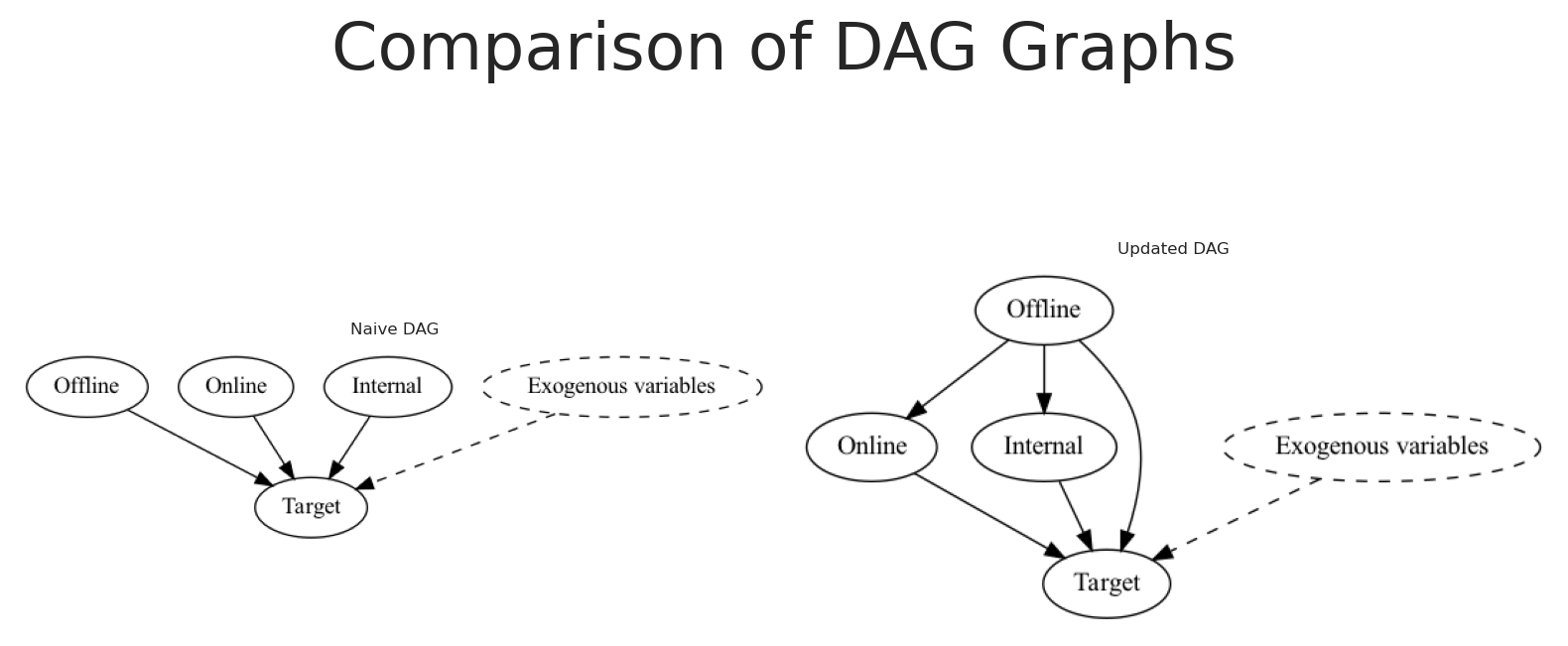
Comprender las independencias condicionales de las variables en nuestro conjunto de datos nos permite identificar los padres de cada variable. Actualmente, hemos identificado que x_3 y x_2 son hijos de x_1, y que x_1 es independiente o verdaderamente exógeno.
Ahora podemos usar esta información para actualizar nuestro grafo causal.
Código
# Initialize a directed graphupdated_naive_causal_mmm_graph = Digraph()# Add nodesupdated_naive_causal_mmm_graph.node("X1", "Offline")updated_naive_causal_mmm_graph.node("X2", "Online")updated_naive_causal_mmm_graph.node("X3", "Internal")updated_naive_causal_mmm_graph.node("E", "Exogenous variables", style="dashed")updated_naive_causal_mmm_graph.node("T", "Target")updated_naive_causal_mmm_graph.edge("E", "T", style="dashed")updated_naive_causal_mmm_graph.edge("X1", "T")updated_naive_causal_mmm_graph.edge("X1","X2")updated_naive_causal_mmm_graph.edge("X1","X3")updated_naive_causal_mmm_graph.edge("X2", "T")updated_naive_causal_mmm_graph.edge("X3", "T")# Create a figure with five subplotsfig, axes = plt.subplots(1, 2,)# Set titles for each subplottitles = ["Naive DAG", "Updated DAG"]for ax, title inzip(axes, titles): ax.set_title(title, fontsize=6) ax.axis('off')# Render and plot each graphnaive_causal_mmm_graph.render(format='png', filename='images/naive_dag')axes[0].imshow(mpimg.imread('images/naive_dag.png'))updated_naive_causal_mmm_graph.render(format='png', filename='images/updated_dag')axes[1].imshow(mpimg.imread('images/updated_dag.png'))# Add main titleplt.suptitle("Comparison of DAG Graphs", fontsize=24)plt.tight_layout()
Genial, podemos actualizar nuestro modelo del mundo para incluir las relaciones causales que hemos identificado. ¿De qué otra manera podemos usar esta información para aprender más sobre las relaciones causales en nuestro conjunto de datos?
Análisis de mediación para el descubrimiento causal
En el análisis de mediación, el efecto total de un predictor X1 sobre un objetivo T se descompone en componentes directos e indirectos. El efecto indirecto opera a través de un mediador M, modelado como M = \alpha_m + a \times X1 + \text{error}. Simultáneamente, el resultado se modela como T = \alpha_y + c' \times X1 + b \times M + \text{error}. Aquí, el producto a \times b cuantifica el efecto indirecto, mientras que c' representa el efecto directo de X1 sobre T. Al estimar estos coeficientes, podemos evaluar si la influencia de X1 sobre T se transmite a través de M, es completamente directa, o una combinación de ambas. La inferencia estadística se realiza usando intervalos credibles, donde los intervalos que excluyen cero indican efectos significativos.
Si el efecto indirecto a \times b es significativo y el efecto directo c' no lo es, concluimos que el impacto de X1 sobre T está completamente mediado por M. Por el contrario, valores significativos tanto para a \times b como para c' sugieren que X1 ejerce influencias directas e indirectas sobre T.
En términos simples, el análisis de mediación nos ayuda a determinar si un predictor X1 influye en un resultado T directamente o principalmente al afectar primero a un mediador M, que luego impacta a T. Si el efecto del mediador es significativo mientras que el efecto directo no lo es, sugiere que X1 afecta a T principalmente a través de su influencia sobre M.
¿Por qué hacer esto sobre el descubrimiento causal que ya hemos realizado? La razón es que podemos usar el análisis de mediación para verificar las relaciones causales que hemos identificado, porque si un nodo es padre del otro, entonces algún efecto está mediado. Si podemos detectar esa mediación, entonces podemos decidir si la relación causal es directa o indirecta. Si no logramos detectar mediación, entonces probablemente nuestros hallazgos no son robustos al descubrimiento causal que hemos realizado.
Código
class MediationAnalysis:""" A class for performing Bayesian mediation analysis using a joint mediation model. The model is specified as: Mediator: M = α_m + a * X + error Outcome: Y = α_y + c′ * X + b * M + error Derived parameters: - Indirect effect: ab = a * b - Total effect: c = c′ + (a * b) Parameters ---------- data : pd.DataFrame DataFrame containing the predictor, mediator, and outcome variables. x : str Column name for the predictor (X). m : str Column name for the mediator (M). y : str Column name for the outcome (Y). hdi : float, optional Credible interval width for HDI (default 0.95). sampler_kwargs : dict, optional Additional keyword arguments for the sampler. Default: {"tune": 1000, "draws": 500, "chains": 4, "random_seed": 42, "target_accept": 0.9, "nuts_sampler": "numpyro", "progressbar": False} """def__init__(self, data: pd.DataFrame, x: str, m: str, y: str, hdi: float=0.95, sampler_kwargs: dict=None):self.data = dataself.x = xself.m = mself.y = yself.hdi = hdiself.sampler_kwargs = sampler_kwargs or {"tune": 1000,"draws": 500,"chains": 4,"random_seed": 42,"target_accept": 0.9,"nuts_sampler": "numpyro","progressbar": False }self.idata =Noneself.model =Nonedef build_model(self):""" Build the Bayesian mediation model. This method constructs the PyMC model and stores it in self.model. Returns ------- model : pm.Model The constructed PyMC model. """# Extract data arrays X_data =self.data[self.x].values M_data =self.data[self.m].values Y_data =self.data[self.y].values N =len(self.data) coords = {"obs": range(N)}with pm.Model(coords=coords) as model:# Mediator path: M = α_m + a * X + error alpha_m = pm.Normal("alpha_m", mu=0.0, sigma=1.0) a = pm.Normal("a", mu=0.0, sigma=1.0) sigma_m = pm.Exponential("sigma_m", lam=1.0) mu_m = alpha_m + a * X_data pm.Normal("M_obs", mu=mu_m, sigma=sigma_m, observed=M_data, dims="obs")# Outcome path: Y = α_y + c′ * X + b * M + error alpha_y = pm.Normal("alpha_y", mu=0.0, sigma=1.0) c_prime = pm.Normal("c_prime", mu=0.0, sigma=1.0) b = pm.Normal("b", mu=0.0, sigma=1.0) sigma_y = pm.Exponential("sigma_y", lam=1.0) mu_y = alpha_y + c_prime * X_data + b * M_data pm.Normal("Y_obs", mu=mu_y, sigma=sigma_y, observed=Y_data, dims="obs")# Derived parameters: indirect and total effects pm.Deterministic("ab", a * b) pm.Deterministic("c", c_prime + a * b)self.model = modeldef fit(self):""" Sample from the previously built mediation model. Returns ------- self : MediationAnalysis The fitted mediation analysis object. Raises ------ ValueError If the model has not been built yet. """ifself.model isNone:raiseValueError("The model has not been built. Call build_model() before fit().")withself.model:self.idata = pm.sample(**self.sampler_kwargs)def get_summary(self):""" Get a numerical summary of the mediation parameters. Returns ------- dict Dictionary with mean estimates and HDI bounds for each parameter. """ var_names = ["alpha_m", "a", "alpha_y", "c_prime", "b", "ab", "c"] summary_df = az.summary(self.idata, var_names=var_names, hdi_prob=self.hdi)# Compute the HDI column names based on the specified interval lower_percent = (1-self.hdi) /2*100 upper_percent =100- lower_percent lower_col =f"hdi_{lower_percent:.1f}%" upper_col =f"hdi_{upper_percent:.1f}%" results = {}for key in var_names: results[key] = {"mean": summary_df.loc[key, "mean"],"hdi_lower": summary_df.loc[key, lower_col],"hdi_upper": summary_df.loc[key, upper_col] }return resultsdef get_report(self, x_label: str=None, m_label: str=None, y_label: str=None):""" Generate a plain-language report of the mediation analysis results. Parameters ---------- x_label : str, optional Label for the predictor variable (default uses self.x). m_label : str, optional Label for the mediator variable (default uses self.m). y_label : str, optional Label for the outcome variable (default uses self.y). Returns ------- str A human-readable summary of the mediation effects. """# Use provided labels or default to variable names x_label = x_label orself.x m_label = m_label orself.m y_label = y_label orself.y var_names = ["a", "b", "c_prime", "ab", "c"] summary_df = az.summary(self.idata, var_names=var_names, hdi_prob=self.hdi)def hdi_includes_zero(row): lower_percent = (1-self.hdi) /2*100 upper_percent =100- lower_percent lower_col =f"hdi_{lower_percent:.1f}%" upper_col =f"hdi_{upper_percent:.1f}%"return row[lower_col] <=0<= row[upper_col]# Extract summary statistics a_stats = summary_df.loc["a"] b_stats = summary_df.loc["b"] c_prime_stats = summary_df.loc["c_prime"] ab_stats = summary_df.loc["ab"] c_stats = summary_df.loc["c"] a_mean = a_stats["mean"] b_mean = b_stats["mean"] c_prime_mean = c_prime_stats["mean"] ab_mean = ab_stats["mean"] c_mean = c_stats["mean"] a_zero = hdi_includes_zero(a_stats) b_zero = hdi_includes_zero(b_stats) c_prime_zero = hdi_includes_zero(c_prime_stats) ab_zero = hdi_includes_zero(ab_stats) c_zero = hdi_includes_zero(c_stats) lines = [] lines.append(f"**Bayesian Mediation Analysis Overview** ({int(self.hdi *100)}% HDI)") lines.append(f"Variables: {x_label} (predictor), {m_label} (mediator), {y_label} (outcome).")# Interpret each pathifnot a_zero: direction ="positive"if a_mean >0else"negative" lines.append(f"- Path a ({x_label} → {m_label}) is credibly {direction} (mean = {a_mean:.3f}).")else: lines.append(f"- Path a ({x_label} → {m_label}) is weak (HDI includes 0, mean = {a_mean:.3f}).")ifnot b_zero: direction ="positive"if b_mean >0else"negative" lines.append(f"- Path b ({m_label} → {y_label}, controlling for {x_label}) is credibly {direction} (mean = {b_mean:.3f}).")else: lines.append(f"- Path b ({m_label} → {y_label}, controlling for {x_label}) is weak (HDI includes 0, mean = {b_mean:.3f}).")ifnot ab_zero: direction ="positive"if ab_mean >0else"negative" lines.append(f"- Indirect effect (a×b) is credibly {direction} (mean = {ab_mean:.3f}).")else: lines.append(f"- Indirect effect (a×b) is uncertain (HDI includes 0, mean = {ab_mean:.3f}).")ifnot c_prime_zero: direction ="positive"if c_prime_mean >0else"negative" lines.append(f"- Direct effect (c') is credibly {direction} (mean = {c_prime_mean:.3f}).")else: lines.append(f"- Direct effect (c') is near zero (HDI includes 0, mean = {c_prime_mean:.3f}).")ifnot c_zero: direction ="positive"if c_mean >0else"negative" lines.append(f"- Total effect (c) is credibly {direction} (mean = {c_mean:.3f}).")else: lines.append(f"- Total effect (c) is uncertain (HDI includes 0, mean = {c_mean:.3f}).") lines.append("")ifnot ab_zero and c_prime_zero: lines.append(f"It appears that {m_label} fully mediates the effect of {x_label} on {y_label} (indirect effect is non-zero while direct effect is near zero).")elifnot ab_zero andnot c_prime_zero: lines.append(f"It appears that {m_label} partially mediates the effect of {x_label} on {y_label} (both indirect and direct effects are credibly non-zero).")else: lines.append("Mediation is unclear or absent (the indirect effect includes zero or the total effect is not clearly different from zero).")return"\n".join(lines)
Ejecutemos el análisis de mediación para las dos primeras variables.
**Bayesian Mediation Analysis Overview** (95% HDI)
Variables: x1 (predictor), x2 (mediator), y (outcome).
- Path a (x1 → x2) is credibly positive (mean = 0.411).
- Path b (x2 → y, controlling for x1) is credibly positive (mean = 0.628).
- Indirect effect (a×b) is credibly positive (mean = 0.258).
- Direct effect (c') is near zero (HDI includes 0, mean = 0.006).
- Total effect (c) is credibly positive (mean = 0.264).

It appears that x2 fully mediates the effect of x1 on y (indirect effect is non-zero while direct effect is near zero).
**Bayesian Mediation Analysis Overview** (95% HDI)
Variables: x1 (predictor), x3 (mediator), y (outcome).
- Path a (x1 → x3) is credibly positive (mean = 0.390).
- Path b (x3 → y, controlling for x1) is credibly positive (mean = 0.359).
- Indirect effect (a×b) is credibly positive (mean = 0.140).
- Direct effect (c') is credibly positive (mean = 0.125).
- Total effect (c) is credibly positive (mean = 0.265).

It appears that x3 partially mediates the effect of x1 on y (both indirect and direct effects are credibly non-zero).
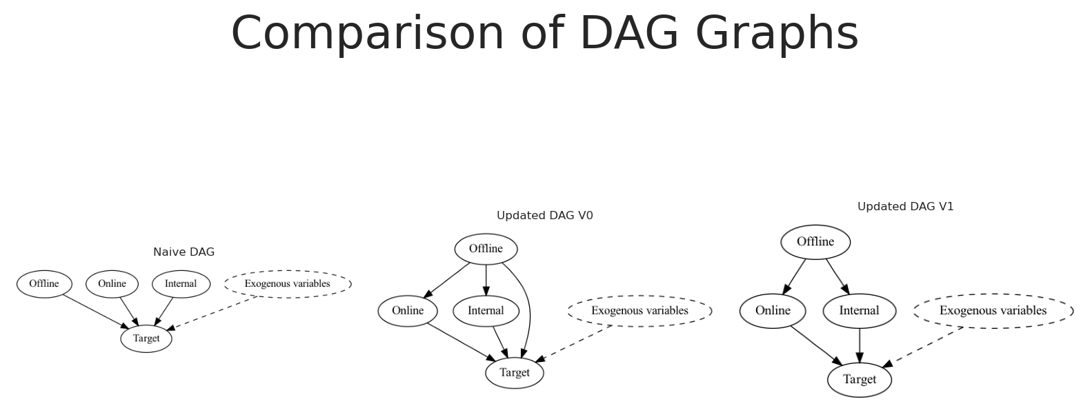
Genial 👏🏻 Basándonos en los siguientes resultados podemos concluir que x_1 afecta a y a través de x_2 y x_3 pero no directamente. Esta conclusión se basa en que el efecto indirecto es significativo y el efecto directo es cercano a cero al controlar por el mediador x2 y parcial para x3.
Si ambos factores estuvieran presentes, el efecto indirecto sería más fuerte, dados los resultados anteriores. Por lo tanto, por simplicidad, no probaremos la mediación cuando ambos factores están presentes.
Podemos nuevamente actualizar nuestro grafo causal para reflejar los nuevos hallazgos.
Código
# Initialize a directed graphupdated_naive_causal_mmm_graph1 = Digraph()# Add nodesupdated_naive_causal_mmm_graph1.node("X1", "Offline")updated_naive_causal_mmm_graph1.node("X2", "Online")updated_naive_causal_mmm_graph1.node("X3", "Internal")updated_naive_causal_mmm_graph1.node("E", "Exogenous variables", style="dashed")updated_naive_causal_mmm_graph1.node("T", "Target")updated_naive_causal_mmm_graph1.edge("E", "T", style="dashed")updated_naive_causal_mmm_graph1.edge("X1","X2")updated_naive_causal_mmm_graph1.edge("X1","X3")updated_naive_causal_mmm_graph1.edge("X2", "T")updated_naive_causal_mmm_graph1.edge("X3", "T")# Create a figure with five subplotsfig, axes = plt.subplots(1, 3,)# Set titles for each subplottitles = ["Naive DAG", "Updated DAG V0", "Updated DAG V1"]for ax, title inzip(axes, titles): ax.set_title(title, fontsize=6) ax.axis('off')# Render and plot each graphnaive_causal_mmm_graph.render(format='png', filename='images/naive_dag')axes[0].imshow(mpimg.imread('images/naive_dag.png'))updated_naive_causal_mmm_graph.render(format='png', filename='images/updated_dag')axes[1].imshow(mpimg.imread('images/updated_dag.png'))updated_naive_causal_mmm_graph1.render(format='png', filename='images/updated_dag1')axes[2].imshow(mpimg.imread('images/updated_dag1.png'))# Add main titleplt.suptitle("Comparison of DAG Graphs", fontsize=24)plt.tight_layout()
¡Esto es genial! Nuestro nuevo grafo causal es más complejo, pero es más preciso que el definido anteriormente. Sin embargo, necesitamos una cantidad significativa de tiempo y trabajo manual para llegar a esta conclusión.
¿Cómo podríamos automatizar este proceso? ¿Es siquiera posible? ¿Y cómo resolvería esto el problema inicial?
¡Sí, es posible! Podemos usar algoritmos de descubrimiento causal para automatizar este proceso.
Introducción al descubrimiento causal
El descubrimiento causal infiere relaciones direccionales de causa y efecto a partir de datos observacionales. Utiliza algoritmos computacionales para construir grafos acíclicos dirigidos que representan posibles mecanismos causales. Estas técnicas se basan en la condición de Markov causal y la suposición de fidelidad estadística. Emplean pruebas estadísticas de independencia condicional para diferenciar las influencias directas de las asociaciones indirectas. Este enfoque integra inferencia estadística y teoría de grafos para modelar sistemas complejos. En general, descubre estructuras causales ocultas que mejoran nuestra comprensión y estimaciones de fenómenos dinámicos.
Suposición de Markov Causal: Cada variable es independiente de sus no-efectos dados sus causas directas, lo que significa que la distribución de probabilidad conjunta puede factorizarse de acuerdo con la estructura del grafo acíclico dirigido. Esto implica que una vez que condicionas sobre las causas inmediatas de una variable, cualquier influencia adicional aguas arriba o paralela se vuelve estadísticamente irrelevante.
Fidelidad Estadística: Esta suposición postula que todas y solo las relaciones de independencia condicional observadas en los datos son las implicadas por el grafo causal. En otras palabras, no hay cancelaciones accidentales ni independencias coincidentes más allá de lo que la estructura causal predice.
Código
class CausalDiscovery:def__init__(self, data):self.data = dataself.labels = [f'{col}'for col in data.columns.to_list()]def greedy_search(self, **kwargs): result = ges(X=self.data.to_numpy(), **kwargs)return result["G"]def peter_clark(self, **kwargs): result = pc(self.data.to_numpy(), **kwargs)return result.Gdef to_pydot(self, graph):return GraphUtils.to_pydot(graph, labels=self.labels)def to_dict(self, graph):""" Convert a general graph to a dictionary representation where each node is a key and the value is a list of its descendants. Parameters ---------- graph : causallearn.graph.GeneralGraph.GeneralGraph The input graph. Returns ------- dict A dictionary where keys are node labels and values are lists of descendant node labels. """ result = {} nodes =sorted(graph.get_nodes(), key=lambda x: str(x))# Initialize the dictionary with empty lists for all nodesfor i, node inenumerate(nodes): result[self.labels[i]] = []# For each node, find its children (direct descendants)for i, node inenumerate(nodes): node_label =self.labels[i]for j, potential_child inenumerate(nodes):if i != j and graph.get_edge(node, potential_child) isnotNone:# Check if there's a directed edge from node to potential_child edge = graph.get_edge(node, potential_child)if (edge.get_endpoint1() == Endpoint.TAIL and edge.get_endpoint2() == Endpoint.ARROW): result[node_label].append(self.labels[j])return resultdef to_graphviz(self, graph, handle_circle="skip"):""" Convert a general graph into a Graphviz Digraph using the pydot conversion for nodes while preserving the original directed edge ordering. Only if the original graph indicates that an edge is undirected (both endpoints are TAIL) do we override the arrow style (using dir="none"). Otherwise, we leave the pydot-provided direction unchanged. Parameters ---------- graph : causallearn.graph.GeneralGraph.GeneralGraph The input graph. handle_circle : str, optional How to handle circle endpoints (not used explicitly here but available for future logic). Returns ------- graphviz.Digraph A Graphviz Digraph where undirected edges are rendered without arrowheads. """# Get the pydot graph (for node positions/labels) dot =self.to_pydot(graph) digraph = Digraph() digraph.attr(size='8,8')# Build a mapping of the original graph nodes based on sorted order. original_nodes =sorted(graph.get_nodes(), key=lambda x: str(x))# Map string indices ("0", "1", …) to the original nodes. index_to_node = {str(i): node for i, node inenumerate(original_nodes)}# Map indices to labels using self.labels. node_labels = {str(i): self.labels[i] for i inrange(len(original_nodes))}# Add nodes to the Graphviz Digraph.for idx_str, label in node_labels.items(): digraph.node(label)# Process each edge from the pydot graph. processed =set() pydot_edges = dot.get_edges()for edge in pydot_edges:# Get source and destination from pydot. src_raw = edge.get_source() dst_raw = edge.get_destination() src_str = src_raw.strip('"') ifisinstance(src_raw, str) elsestr(src_raw) dst_str = dst_raw.strip('"') ifisinstance(dst_raw, str) elsestr(dst_raw)# Get original node objects using our mapping. src_node = index_to_node.get(src_str) dst_node = index_to_node.get(dst_str)if src_node isNoneor dst_node isNone:continue# Get display labels. src_label = node_labels.get(src_str, src_str) dst_label = node_labels.get(dst_str, dst_str)# Use a tuple (src_str, dst_str) to ensure we don't add duplicates. edge_key = (src_str, dst_str) reverse_key = (dst_str, src_str)if edge_key in processed or reverse_key in processed:continuetry:# Get endpoint information from the original graph. e_uv = graph.get_endpoint(src_node, dst_node) e_vu = graph.get_endpoint(dst_node, src_node)exceptKeyError:# Skip if the original graph doesn't contain this edge.continue# If both endpoints are TAIL, we treat the edge as undirected.if e_uv == Endpoint.TAIL and e_vu == Endpoint.TAIL: digraph.edge(src_label, dst_label, dir="none") processed.add(edge_key) processed.add(reverse_key)else:# Otherwise, preserve the original pydot direction. digraph.edge(src_label, dst_label) processed.add(edge_key)return digraphdef to_networkx(self, graph) -> nx.DiGraph:""" Convert a general graph (e.g. from causallearn) into a NetworkX DiGraph. Nodes are added as provided by graph.get_nodes(), and for each ordered pair (u, v) where an edge exists (as determined by graph.get_endpoint(u, v)), we add a directed edge with an attribute 'endpoint' that stores the edge marker. If the general graph does not provide a direct list of edges (e.g. via a get_edges() method), we iterate over all pairs of nodes. """ digraph = nx.DiGraph() nodes = graph.get_nodes()# Add nodes to the networkx graph.for node in nodes: digraph.add_node(node)# If available, use a dedicated method to get edges.try: edges = graph.get_edges()exceptAttributeError:# Fallback: iterate over all ordered pairs (inefficient for large graphs) edges = []for u in nodes:for v in nodes:if u == v:continuetry:# Attempt to get an endpoint; if present, we consider that an edge exists. _ = graph.get_endpoint(u, v) edges.append((u, v))exceptKeyError:continue# Add edges with endpoint attributes.for u, v in edges:try: endpoint_uv = graph.get_endpoint(u, v)exceptKeyError:continue digraph.add_edge(u, v, endpoint=endpoint_uv)return digraphdef _networkx_to_graphviz(self, nx_graph: nx.DiGraph) -> Digraph:""" Convert a NetworkX DiGraph into a Graphviz Digraph. This method uses similar logic to 'to_graphviz', checking for reciprocal edges. If an edge (u,v) and its reverse (v,u) exist and both have the attribute endpoint equal to Endpoint.TAIL, the edge is rendered as undirected (dir="none"). """ digraph = Digraph() digraph.attr(size='8,8') processed =set()# Sort nodes to create a consistent mapping with self.labels. sorted_nodes =sorted(nx_graph.nodes(), key=lambda x: str(x)) node_labels = {}for i, node inenumerate(sorted_nodes):# Use self.labels if available, otherwise default to the node's string representation. label =self.labels[i] if i <len(self.labels) elsestr(node) node_labels[node] = label digraph.node(label)for u, v in nx_graph.edges():if (u, v) in processed or (v, u) in processed:continue src_label = node_labels.get(u, str(u)) dst_label = node_labels.get(v, str(v))# Check if the reverse edge exists to potentially mark as undirected.if nx_graph.has_edge(v, u): endpoint_uv = nx_graph.edges[u, v].get('endpoint', None) endpoint_vu = nx_graph.edges[v, u].get('endpoint', None)if endpoint_uv == Endpoint.TAIL and endpoint_vu == Endpoint.TAIL: digraph.edge(src_label, dst_label, dir="none") processed.add((u, v)) processed.add((v, u))continue# Otherwise, add the edge as directed. digraph.edge(src_label, dst_label) processed.add((u, v))return digraphdef _graphviz_to_networkx(self, gv_graph: Digraph) -> nx.DiGraph:""" Convert a Graphviz Digraph into a NetworkX DiGraph. This method extracts the DOT source from the provided Graphviz Digraph, parses it using pydot, and then converts the resulting pydot graph into a NetworkX directed graph. This ensures that node labels and edge orientations are maintained consistently. Parameters ---------- gv_graph : graphviz.Digraph The Graphviz Digraph to be converted. Returns ------- nx.DiGraph A NetworkX DiGraph representation of the input Graphviz graph. """# Retrieve the DOT source code from the Graphviz Digraph. dot_str = gv_graph.source# Parse the DOT data using pydot. pydot_graphs = pydot.graph_from_dot_data(dot_str)ifnot pydot_graphs:raiseValueError("No valid pydot graphs could be parsed from the DOT data.")# pydot.graph_from_dot_data returns a list; we take the first one. pydot_graph = pydot_graphs[0]# Use NetworkX’s built-in conversion from a pydot graph to a DiGraph. nx_graph = nx.nx_pydot.from_pydot(pydot_graph)return nx_graph
Causal Learn nos permite usar diferentes algoritmos para inferir la clase equivalente de Markov del grafo causal. La clase anterior es un wrapper que nos permite usar los diferentes algoritmos implementados en la biblioteca causal learn, y graficarlos más fácilmente.
Actualmente incluimos los siguientes algoritmos:
Búsqueda Voraz (GES)
Peter-Clark (PC)
Algoritmos de Descubrimiento Causal
El algoritmo Peter-Clark es un método basado en restricciones que infiere estructuras causales a partir de datos observacionales usando pruebas de independencia condicional. Comienza con un grafo completamente conectado no dirigido donde cada variable está inicialmente conectada a todas las demás. El algoritmo prueba sistemáticamente la independencia condicional entre pares de variables, condicionando sobre subconjuntos cada vez más grandes de otras variables. Cuando se detecta una independencia condicional, la arista correspondiente se elimina del grafo.
Por otro lado, Búsqueda Voraz es un método basado en puntuación que mejora iterativamente un modelo causal candidato modificando localmente su estructura. Comienza con un grafo acíclico dirigido inicial y evalúa una métrica de puntuación que equilibra el ajuste con la complejidad del modelo. El algoritmo explora modificaciones como agregar, eliminar o invertir aristas para encontrar mejoras locales en la puntuación. En cada iteración, selecciona el cambio que produce el mayor aumento en la puntuación, siguiendo una estrategia de mejora paso a paso. La búsqueda continúa hasta que ninguna modificación individual puede mejorar más la puntuación del modelo. Este método navega eficientemente por el espacio de búsqueda combinatorio de grafos posibles mediante decisiones localmente óptimas.
Suposición de Suficiencia Causal
Suposición de Suficiencia Causal
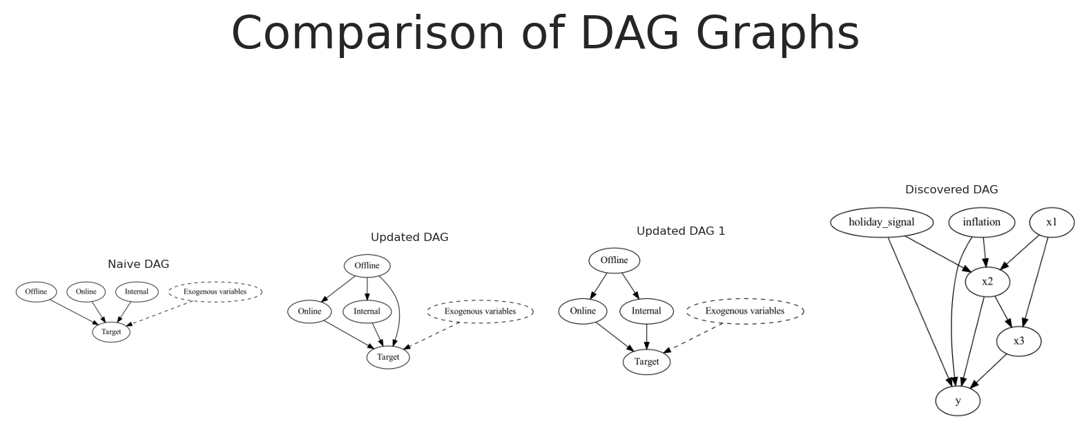
El siguiente ejemplo muestra el grafo causal inferido usando el algoritmo de Búsqueda Voraz.
Código
causal_model = CausalDiscovery(scaled_df[["holiday_signal", "inflation", "x1", "x2", "x3", "y"]])ges_graph = causal_model.greedy_search()# Create a figure with five subplotsfig, axes = plt.subplots(1, 4,)# Set titles for each subplottitles = ["Naive DAG", "Updated DAG", "Updated DAG 1", "Discovered DAG"]for ax, title inzip(axes, titles): ax.set_title(title, fontsize=6) ax.axis('off')# Render and plot each graphnaive_causal_mmm_graph.render(format='png', filename='images/naive_dag')axes[0].imshow(mpimg.imread('images/naive_dag.png'))updated_naive_causal_mmm_graph.render(format='png', filename='images/updated_dag')axes[1].imshow(mpimg.imread('images/updated_dag.png'))updated_naive_causal_mmm_graph1.render(format='png', filename='images/updated_dag1')axes[2].imshow(mpimg.imread('images/updated_dag1.png'))real_dag_graph = causal_model.to_graphviz(ges_graph)real_dag_graph.render(format='png', filename='images/discovered_dag')axes[3].imshow(mpimg.imread('images/discovered_dag.png'))# Add main titleplt.suptitle("Comparison of DAG Graphs", fontsize=24)plt.tight_layout()
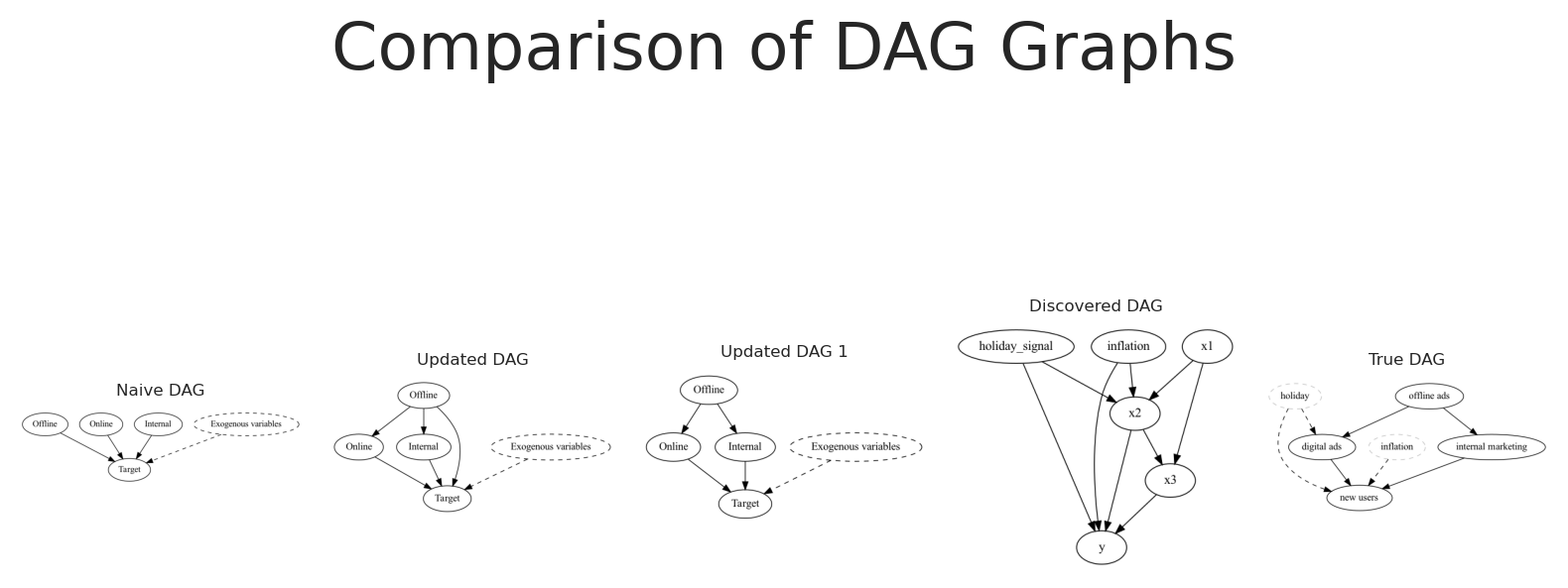
El grafo causal capturado por la búsqueda voraz es muy similar al grafo causal verdadero. Algunas flechas apuntan a variables que no están relacionadas, pero esto es esperado dada la naturaleza de los datos: aún tenemos ruido en los datos y correlaciones espurias que no pueden ser completamente falsificadas por las pruebas de independencia. Además, el grafo encontrado puede estar en la clase equivalente de Markov del grafo causal verdadero, lo que significa que hay múltiples DAGs compatibles con los datos.
En lugar de ser un problema, esto es una gran noticia porque ahora podemos empezar a trabajar con experimentación para probar la estructura actual, y mejorarla de forma iterativa, sin necesidad de esperar a estas respuestas para obtener las estimaciones correctas en un modelo de regresión.
Desglosemos las vías causales de x2 a y en el grafo:
Vías de confusión:
Día festivo: Afecta tanto a x2 como a y (holiday → x2 y holiday → y).
Inflación: Afecta tanto a x2 como a y (inflation → x2 y inflation → y).
x1: Influye en x2 (x1 → x2) y también afecta a y indirectamente a través de x3 (x1 → x3 → y).
Vía de mediación:
x3: Se encuentra en la vía causal de x2 a y (x2 → x3 → y).
¿Qué necesita ser controlado?
Para estimar el efecto total de x2 sobre y sin sesgo, necesitas bloquear todas las vías de retroceso (confusión). Esto significa controlar por las causas comunes:
Día festivo
Inflación
x1
¿Por qué no controlar por x3? Dado que x3 es un mediador (es decir, transmite parte del efecto de x2 a y), incluirlo en tu regresión bloquearía el efecto indirecto de x2 sobre y. Este “sobre-control” resultaría en una estimación que refleja solo el efecto directo de x2 sobre y, no el efecto total. Además, controlar por mediadores puede a veces introducir sesgo si existen otras relaciones complejas en el grafo.
There were 24 divergences after tuning. Increase `target_accept` or reparameterize.
Sampling: [y]
Ahora grafiquemos la distribución posterior del efecto de x3 sobre y.
Código
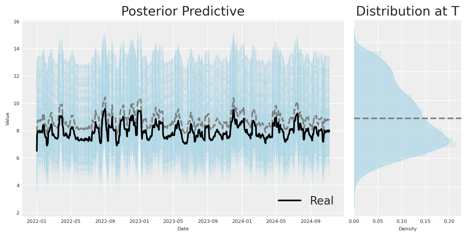
def plot_posterior(y_real, posterior, figsize=(8, 4), path_color='orange', hist_color='orange', **kwargs):""" Plot the posterior distribution of a stochastic process. Parameters ---------- y_real : array-like The real values to compare against the posterior. posterior : xarray.DataArray The posterior distribution with shape (draw, chain, date). figsize : tuple, optional Size of the figure. Default is (8, 4). path_color : str, optional Color of the paths in the time series plot. Default is 'orange'. hist_color : str, optional Color of the histogram. Default is 'orange'. **kwargs : dict Additional keyword arguments to pass to the plotting functions. Returns ------- fig : matplotlib.figure.Figure The figure object containing the plots. """# Calculate the expected value (mean) across all draws and chains for each date expected_value = posterior.mean(dim=("draw", "chain"))# Create a figure and a grid of subplots fig = plt.figure(figsize=figsize) gs = fig.add_gridspec(1, 2, width_ratios=[3, 1])# Time series plot ax1 = fig.add_subplot(gs[0])for chain inrange(posterior.shape[1]):for draw inrange(0, posterior.shape[0], 10): # Plot every 10th draw for performance ax1.plot(posterior.date, posterior[draw, chain], color=path_color, alpha=0.1, linewidth=0.5) ax1.plot(posterior.date, expected_value, color='grey', linestyle='--', linewidth=2) ax1.plot(posterior.date, y_real, color='black', linestyle='-', linewidth=2, label='Real',) ax1.set_title("Posterior Predictive") ax1.set_xlabel('Date') ax1.set_ylabel('Value') ax1.grid(True) ax1.legend()# KDE plot ax2 = fig.add_subplot(gs[1]) final_values = posterior[:, :, -1].values.flatten()# Use seaborn for KDE plot sns.kdeplot(y=final_values, ax=ax2, fill=True, color=hist_color, alpha=0.6, **kwargs)# Add histogram on top of KDE ax2.hist(final_values, orientation='horizontal', color=hist_color, bins=30, alpha=0.3, density=True) ax2.axhline(y=expected_value[-1], color='grey', linestyle='--', linewidth=2) ax2.set_title('Distribution at T') ax2.set_xlabel('Density') ax2.set_yticklabels([]) # Hide y tick labels to avoid duplication ax2.grid(True)return figplot_posterior( df["x3_adstock_saturated"].values, mmm.idata.posterior.channel_contribution.sel(channel="x3") * df["y"].max(), path_color='lightblue', hist_color='lightblue');
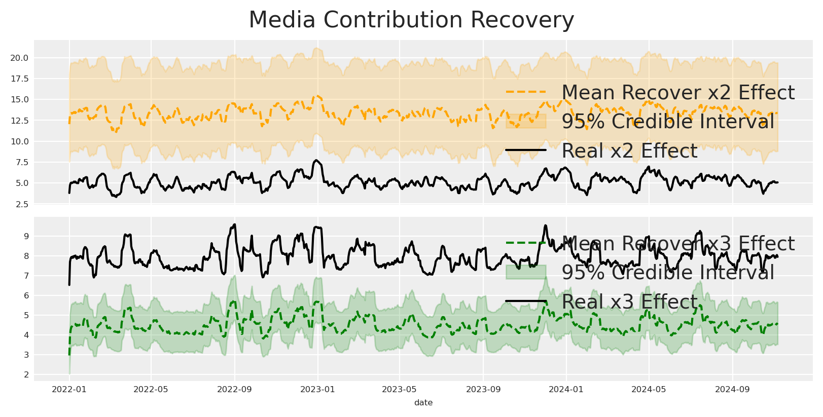
El efecto se recuperó perfectamente. Usando este modelo, podemos informar de forma segura cuánto obtendremos si invertimos en x3. Sin embargo, necesitamos controlar por día festivo e inflación para obtener el efecto total. ¿Qué pasa si no tenemos estas variables de control?
¿Cómo obtener estimaciones correctas si no tenemos todas las covariables?
Si estamos seguros de nuestro proceso generativo de datos, podemos estar seguros de que al excluir quirúrgicamente un nodo, un proceso gaussiano puede absorber tal variabilidad. Veamos cómo funciona esto en la práctica.
The rhat statistic is larger than 1.01 for some parameters. This indicates problems during sampling. See https://arxiv.org/abs/1903.08008 for details
The effective sample size per chain is smaller than 100 for some parameters.  A higher number is needed for reliable rhat and ess computation. See https://arxiv.org/abs/1903.08008 for details
Sampling: [y]
mean
sd
hdi_3%
hdi_97%
mcse_mean
mcse_sd
ess_bulk
ess_tail
r_hat
saturation_alpha[x1]
0.291
0.064
0.173
0.404
0.003
0.001
462.0
443.0
1.00
saturation_alpha[x2]
0.821
0.028
0.772
0.874
0.001
0.001
498.0
816.0
1.01
saturation_lam[x1]
1.944
0.558
0.938
2.946
0.023
0.011
514.0
575.0
1.00
saturation_lam[x2]
0.418
0.026
0.370
0.468
0.001
0.001
444.0
558.0
1.01
adstock_alpha[x1]
0.448
0.046
0.362
0.534
0.002
0.001
832.0
1379.0
1.01
adstock_alpha[x2]
0.325
0.020
0.290
0.366
0.001
0.000
729.0
1754.0
1.01
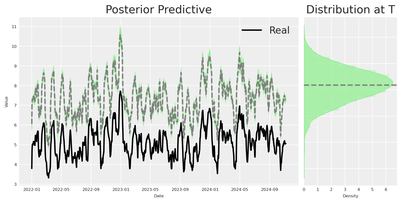
Podemos ver por los parámetros del modelo que es capaz de recuperar el efecto de x2 sobre y, aunque eliminamos x3 del modelo.
Como se esperaba, el efecto de x2 sobre y se recupera, aunque eliminamos las variables de control del modelo y usamos un proceso gaussiano para explicar la variabilidad de los datos en su lugar.
Conclusiones
No busques un único modelo: El mundo real es muy dinámico, es posible que el único modelo no exista.
“Encuentra” la Verdad Causal: Sumérgete en el mundo de las estructuras causales y aprende a mapear los caminos ocultos que influyen en tus resultados. No considerar las estructuras causales te llevará a considerar estructuras más simples, lo cual puede ser problemático en un entorno del mundo real.
Abraza la Evolución del Modelo: ¡No te aferres demasiado a tu primer modelo! Como vimos en nuestra progresión de DAGs, los modelos pueden (y deben) cambiar a medida que aprendemos más. Empezar simple está bien, pero prepárate para elevar el nivel de tu modelo cuando los datos muestren que hay más en la historia.
Nuestro proceso de descubrimiento causal en pocas palabras
A lo largo del cuaderno, hemos visto cómo podemos usar modelos de regresión Bayesiana para identificar la estructura causal de un conjunto de datos, y cómo podemos usar esta información para tomar mejores decisiones. También hemos visto cómo podemos usar esta información para tomar mejores decisiones. En resumen, empezamos con una comprensión ingenua y simple del mundo, que fue evolucionando a través de la identificación de la estructura causal de los datos, y el uso del grafo causal para tomar mejores decisiones de modelado.
Código
# Create a figure with five subplotsfig, axes = plt.subplots(1, 5,)# Set titles for each subplottitles = ["Naive DAG", "Updated DAG", "Updated DAG 1", "Discovered DAG", "True DAG"]for ax, title inzip(axes, titles): ax.set_title(title, fontsize=6) ax.axis('off')# Render and plot each graphnaive_causal_mmm_graph.render(format='png', filename='images/naive_dag')axes[0].imshow(mpimg.imread('images/naive_dag.png'))updated_naive_causal_mmm_graph.render(format='png', filename='images/updated_dag')axes[1].imshow(mpimg.imread('images/updated_dag.png'))updated_naive_causal_mmm_graph1.render(format='png', filename='images/updated_dag1')axes[2].imshow(mpimg.imread('images/updated_dag1.png'))real_dag_graph = causal_model.to_graphviz(ges_graph)real_dag_graph.render(format='png', filename='images/discovered_dag')axes[3].imshow(mpimg.imread('images/discovered_dag.png'))new_real_dag.render(format='png', filename='images/true_dag')axes[4].imshow(mpimg.imread('images/true_dag.png'))# Add main titleplt.suptitle("Comparison of DAG Graphs", fontsize=24)plt.tight_layout()
---title: "Baby Steps for Causal Discovery"author: "Carlos Trujillo"date: "2025-02-01"description: "An introduction to causal discovery for marketing and data science, presented at PyData Tallinn 2025."categories: [python, experimentation, media mix modeling, mmm, bayesian, pymc, causal discovery, causal learning, pydata, tallinn, estonia]image: "/images/baby_steps_for_causal_discovery.jpg"image-alt: "Causal discovery graph introduction for marketing and data science applications"jupyter: baby_steps_for_causal_discoveryformat: html: code-fold: true code-tools: true code-overflow: wrap---# Introduction to Causal DiscoveryIn this notebook, we'll dive into how to uncover causal relationships in marketing data, a crucial step for understanding the true impact of various channels on business outcomes. We'll start by generating synthetic data that mimics real-world marketing scenarios, complete with confounding variables and complex causal structures.Next, we'll fit a Bayesian marketing mix model using PyMC-Marketing, check causal directions between variables, and perform mediation analysis to explore indirect effects. Finally, we'll use structure discovery techniques to infer potential causal graphs. By the end, you'll have a solid grasp of how to apply these techniques to reveal hidden causal insights in your marketing data.```{python}import warningswarnings.filterwarnings("ignore")from pymc_marketing.mmm.transformers import geometric_adstock, michaelis_mentenfrom pymc_marketing.mmm import MMM, GeometricAdstock, MichaelisMentenSaturationfrom pymc_extras.prior import Priorimport networkx as nxfrom graphviz import Digraphimport pydotimport arviz as azimport matplotlib.pyplot as pltimport matplotlib.image as mpimgimport seaborn as snsfrom IPython.display import SVG, displayimport numpy as npimport pandas as pdimport preliz as pzimport pymc as pmfrom PIL import Imagefrom io import BytesIOfrom causallearn.graph.Endpoint import Endpointfrom causallearn.utils.GraphUtils import GraphUtilsfrom causallearn.search.ScoreBased.GES import gesfrom causallearn.search.ConstraintBased.PC import pcaz.style.use("arviz-darkgrid")plt.rcParams["figure.figsize"] = [8, 4]plt.rcParams["figure.dpi"] =100plt.rcParams["axes.labelsize"] =6plt.rcParams["xtick.labelsize"] =6plt.rcParams["ytick.labelsize"] =6plt.rcParams.update({"figure.constrained_layout.use": True})%load_ext autoreload%autoreload 2%config InlineBackend.figure_format ="retina"seed =sum(map(ord, "Estimating effects despite having Confounding Variables"))rng = np.random.default_rng(seed)print(seed)print(rng)```# Business caseAs a company we probably invest in different channels to acquire new customers. Some actions are more direct, like paid ads, and others are more indirect, like offline media marketing, as marketers and scientist, we want to understand the impact of each channel on the target variable (number of new customers).The following DAG shows a possible causal structure of the problem. Let's say we have the following variables:- $x1$: offline ads, e.g. TV, radio, print, etc.- $x2$: digital ads, e.g. SEM, SEO, social media, etc.- $x3$: internal marketing, e.g. product marketing, internal communication, etc.- $y$: new usersIts probable that our offline ads are not directly affecting our new users, but they are affecting our digital ads and internal marketing, users observe a banner of our product and then they search for it online or they are referred by a friend which finally converts using their phone. Independently, some digital ads can impact users which haven't heard of us before, and those could convert directly.On top of that, we have some external factors that could affect our new users, e.g. holidays, economic conditions, etc. Things like holidays could affect even more our digital ads, e.g. more users are online shopping, and we are investing more during those days as well.This creates a complex causal structure, where variables are not fully independent and it is not easy to infer the causal impact of each channel on the target variable.```{python}new_real_dag = Digraph(comment='DAG')new_real_dag.node('z', 'holiday', color='grey', style='dashed')new_real_dag.node('m', 'inflation', color='grey', style='dashed')new_real_dag.node('x1', 'offline ads')new_real_dag.node('x2', 'digital ads')new_real_dag.node('x3', 'internal marketing')new_real_dag.node('y', 'new users')new_real_dag.edge('z', 'x2', style='dashed')new_real_dag.edge('x1', 'x2')new_real_dag.edge('x1', 'x3')new_real_dag.edge('z', 'y', style='dashed')new_real_dag.edge('x2', 'y')new_real_dag.edge('x3', 'y')new_real_dag.edge('m', 'y', style='dashed')new_real_dag```## Data generationBased on the provided DAG, we can create some synthetic data to test how our model performs when we have a complex causal structures. Using the same data, we can test different model compositions and see how could we improve our model to uncover the true causal impact of each channel on the target variable.We'll start by setting the date range. Here we'll use a date range from 2022-01-01 to 2024-11-06, meaning we have almost 3 years of data (1041 days).```{python}# date rangemin_date = pd.to_datetime("2022-01-01")max_date = pd.to_datetime("2024-11-06")date_range = pd.date_range(start=min_date, end=max_date, freq="D")df = pd.DataFrame(data={"date_week": date_range}).assign( year=lambda x: x["date_week"].dt.year, month=lambda x: x["date_week"].dt.month, dayofyear=lambda x: x["date_week"].dt.dayofyear,)n = df.shape[0]print(f"Number of observations: {n}")```### Holiday signalCertain holidays, like Christmas, can have a significant impact on consumer behavior before and after the specific date, leading to seasonal spikes in sales. To capture these effects, we introduce a holiday signal based on Gaussian (normal) distributions centered around specific holiday dates.The function used to model the holiday effect is defined as follows:$$H_{t} = \exp\left(-0.5 \left(\frac{\Delta t}{\sigma}\right)^2\right)$$Where:- $\Delta t$ is the time difference (in days) between the current date and the holiday date.- $\sigma$ is the standard deviation that controls the spread of the effect around the holiday date.For each holiday, we calculate the holiday signal across the date range and add a **holiday contribution** by scaling the signal with a holiday-specific coefficient. This approach models seasonal holiday spikes using Gaussian functions, which capture the transient increase in market activity around holidays, and their respective decay over time.> Note: Here we assume a normally distributed signal, nevertheless the signal could be skew or not normal distributed.```{python}holiday_dates = ["24-12", "31-12", "08-06", "07-09"] # List of holidays as month-day stringsstd_devs = [5, 5, 3, 3] # List of standard deviations for each holidayholidays_coefficients = [2, 3, 4, 6]# Initialize the holiday effect arrayholiday_signal = np.zeros(len(date_range))holiday_contributions = np.zeros(len(date_range))# Generate holiday signalsfor holiday, std_dev, holiday_coef inzip( holiday_dates, std_devs, holidays_coefficients, strict=False):# Find all occurrences of the holiday in the date range holiday_occurrences = date_range[date_range.strftime("%d-%m") == holiday]for occurrence in holiday_occurrences:# Calculate the time difference in days time_diff = (date_range - occurrence).days# Generate the Gaussian basis for the holiday _holiday_signal = np.exp(-0.5* (time_diff / std_dev) **2)# Add the holiday signal to the holiday effect holiday_signal += _holiday_signal holiday_contributions += _holiday_signal * holiday_coefdf["holiday_signal"] = holiday_signaldf["holiday_contributions"] = holiday_contributions# Plot the holiday effectfig, ax = plt.subplots()sns.lineplot(x=date_range, y=holiday_signal, ax=ax)ax.set(title="Holiday Effect Signal", xlabel="Date", ylabel="Signal Intensity")plt.show()```### Generating inflationNext, we generate the data for **Inflation**. We assume the inflation follows a power-law trend, meaning that growth accelerates over time rather than remaining constant. This can be mathematically defined as:$$IN_{t} = (t + \text{baseline})^{\text{exponent}} - 1$$Where:- $t$: The time index, representing days since the start of the date range.- $baseline$: A constant added to $t$ to shift the starting point of the trend. This value affects the initial level of market growth. The starting value of the function will be $(baseline)^{exponent} - 1$, not 0.- $exponent$: The power to which the time index is raised, determining the rate at which the trend accelerates over time.```{python}df["inflation"] = (np.linspace(start=0.0, stop=50, num=n) +10) ** (2/4) -1fig, ax = plt.subplots()sns.lineplot( x="date_week", y="inflation", color="C2", label="trend", data=df, ax=ax)ax.legend(loc="upper left")ax.set(title="Inflation Components", xlabel="date", ylabel=None);```### Modeling Marketing ChannelsIn this section, we simulate three marketing channels, $x1$, $x2$, and $x3$ which represent different advertising channels (e.g., Internal Marketing, Social Marketing, Offline Marketing). Each channel's behavior is influenced by random variability and confounding effects from seasonal holidays. Here’s how we model each channel mathematically:**Channel $x1$**:As mentioned before, we generate $x1$ which is affected by the holiday signal, we could define it as:$$I_{x1_t} = S_{x1_t} + e_{x1}$$**Channel $x2$**:On the other hand, we generate $x2$ which is affected by the holiday signal, and the influence of $x1$. We could define it as:$$I_{x2_t} = S_{x2_t} + H_{t} \times \alpha_{x2} + (I_{x1_t} \times \alpha_{x1_x2}) + e_{x2}$$**Channel $x3$**:For the last variable, we generate $x3$ which is affected by $x1$ only.$$I_{x3_t} = S_{x3_t} + (I_{x1_t} \times \alpha_{x1_x3}) + e_{x3}$$These equations allow us to capture the complex dynamics influencing each marketing channel:- **Holiday Effects** increase channel activity around specific dates, simulating seasonal spikes.- **Cross-channel Influences** introduce interdependencies, modeling how one channel's success can amplify another’s.> Note: Here we are assuming an additive impact for the channel interactions.```{python}x1 = pz.Gamma(mu=1, sigma=3).rvs(n, random_state=rng)cofounder_effect_holiday_x1 =2.5x1_conv = np.convolve(x1, np.ones(14) /14, mode="same")noise = pz.Normal(mu=0, sigma=0.1).rvs(28, random_state=rng)x1_conv[:14] = x1_conv.mean() + noise[:14]x1_conv[-14:] = x1_conv.mean() + noise[14:]df["x1"] = x1_convx2 = pz.Gamma(mu=2, sigma=2).rvs(n, random_state=rng)cofounder_effect_holiday_x2 =2.2cofounder_effect_x1_x2 =1.3x2_conv = np.convolve(x2, np.ones(18) /12, mode="same")noise = pz.Normal(mu=0, sigma=0.1).rvs(28, random_state=rng)x2_conv[:14] = x2_conv.mean() + noise[:14]x2_conv[-14:] = x2_conv.mean() + noise[14:]df["x2"] = ( x2_conv+ (holiday_signal * cofounder_effect_holiday_x2)+ (df["x1"] * cofounder_effect_x1_x2)) # digital adsx3 = pz.Gamma(mu=5, sigma=1).rvs(n, random_state=rng)cofounder_effect_x1_x3 =1.5x3_conv = np.convolve(x3, np.ones(16) /10, mode="same")noise = pz.Normal(mu=0, sigma=0.1).rvs(28, random_state=rng)x3_conv[:14] = x3_conv.mean() + noise[:14]x3_conv[-14:] = x3_conv.mean() + noise[14:]df["x3"] = ( x3_conv+ (df["x1"] * cofounder_effect_x1_x3)) # internal marketing```We'll assume all of marketing activities suffer the same transformations Adstock and Saturation. This means, each channel will have individual parameters for the selected transformations, in this case Geometrick adstock and michaelis menten.```{python}# apply geometric adstock transformationalpha2: float=0.4alpha3: float=0.3df["x2_adstock"] = ( geometric_adstock(x=df["x2"].to_numpy(), alpha=alpha2, l_max=24, normalize=True) .eval() .flatten())df["x3_adstock"] = ( geometric_adstock(x=df["x3"].to_numpy(), alpha=alpha3, l_max=24, normalize=True) .eval() .flatten())# apply saturation transformationlam2: float=6.0lam3: float=12.0alpha_mm2: float=12alpha_mm3: float=18df["x2_adstock_saturated"] = michaelis_menten( x=df["x2_adstock"].to_numpy(), lam=lam2, alpha=alpha_mm2)df["x3_adstock_saturated"] = michaelis_menten( x=df["x3_adstock"].to_numpy(), lam=lam3, alpha=alpha_mm3)fig, ax = plt.subplots( nrows=3, ncols=2, sharex=True, sharey=False, layout="constrained")sns.lineplot(x="date_week", y="x2", data=df, color="C1", ax=ax[0, 0])sns.lineplot(x="date_week", y="x3", data=df, color="C2", ax=ax[0, 1])sns.lineplot(x="date_week", y="x2_adstock", data=df, color="C1", ax=ax[1, 0])sns.lineplot(x="date_week", y="x3_adstock", data=df, color="C2", ax=ax[1, 1])sns.lineplot(x="date_week", y="x2_adstock_saturated", data=df, color="C1", ax=ax[2, 0])sns.lineplot(x="date_week", y="x3_adstock_saturated", data=df, color="C2", ax=ax[2, 1])fig.suptitle("Media Costs Data - Transformed", fontsize=16)# adjust size of X axisax[2, 0].tick_params(axis="x", labelsize=8)ax[2, 1].tick_params(axis="x", labelsize=8)# adjust size of x axis labelsfor ax in ax.flat: ax.tick_params(axis="x", labelsize=6)```The previous plot shows how the transformations affect each variable, and what would be the true contribution after each transformation.### Target variableThe target variable is a combination of all variables before. The mathematical formula can be expressed as:$$y_{t} = Intercept - f(IN_{t}) + f(H_{t}) + m(I_{x3_t}) + m(I_{x2_t}) + \epsilon$$Where:- **Intercept**: A baseline level of sales, set to 1.5, representing the base sales level in the absence of other effects.- **Inflation**: Represents the underlying market inflation, with an implicit negative coefficient of 1, adding a steady downward influence.- **Holiday Contributions**: Adds sales spikes around holiday periods, capturing the seasonal increase in consumer demand.- **$m(Impressions_{x3_t})$ and $m(Impressions_{x2_t})$**: Represent the **saturated adstock** values for the marketing channels $x3$ and $x2$.- **Noise $\epsilon$**: A small random error term, drawn from a normal distribution with mean 0 and standard deviation 0.08, to account for unexplained variability in sales.```{python}df["intercept"] =1.5df["epsilon"] = rng.normal(loc=0.0, scale=0.08, size=n)df["y"] = ( df["intercept"]+ df["holiday_contributions"]+ df["x2_adstock_saturated"]+ df["x3_adstock_saturated"]+ df["epsilon"] # Noise) - df["inflation"]fig, ax = plt.subplots()sns.lineplot(x="date_week", y="y", color="black", data=df, ax=ax)ax.set(title="Sales (Target Variable)", xlabel="date", ylabel="y (thousands)");```We can scale the full dataset and we'll have finally something very similar to reality.```{python}# scale df by abs max per columndf["date"] = pd.to_datetime(df["date_week"])scaled_df = df.copy()for col in scaled_df.columns:if col !='date'and col !='date_week': scaled_df[col] = scaled_df[col] / scaled_df[col].abs().max()scaled_df[["date", "x1", "x2", "x3", "y"]].head()```# Intial approachIf we have a dataset like the one we just created, we can try to fit a model with the following to find the causal impact of each channel on the target variable. For the example, we'll use a simple model from Pymc-Marketing for this purpose.Let's see what happens if we fit a model with all what we have without any knowledge of the causal structure.```{python}scaled_df[["date", "x1", "x2", "x3", "y"]].head()model_config = {"intercept": Prior("Gamma", mu=1, sigma=1),"likelihood": Prior("Normal", sigma=Prior("Normal", mu=0, sigma=.5)),}fit_kwargs =dict(nuts_sampler="numpyro", random_seed=rng,)X = df.drop(columns=["y"])y = df["y"]mmm = MMM( date_column="date", channel_columns=["x1","x2","x3" ], control_columns=["holiday_signal","inflation" ], adstock=GeometricAdstock(l_max=24), saturation=MichaelisMentenSaturation(),)mmm.fit(X, y, **fit_kwargs)mmm.sample_posterior_predictive( X=X, extend_idata=True, combined=True, random_seed=rng,)```How the recover contributions look like, If we compare to the real contributions?```{python}initial_model_recover_effect = ( az.hdi(mmm.fit_result["channel_contribution"], hdi_prob=0.95)* mmm.target_transformer["scaler"].scale_.item())initial_model_mean_effect = ( mmm.fit_result.channel_contribution.mean(dim=["chain", "draw"])* mmm.target_transformer["scaler"].scale_.item())fig, ax = plt.subplots(2, 1, sharex=True)# x2 -> onlineax[0].plot( date_range, initial_model_mean_effect.sel(channel="x2"), label="Mean Recover x2 Effect", linestyle="--", color="orange",)ax[0].fill_between( date_range, initial_model_recover_effect.channel_contribution.isel(hdi=0).sel(channel="x2"), initial_model_recover_effect.channel_contribution.isel(hdi=1).sel(channel="x2"), alpha=0.2, label="95% Credible Interval", color="orange",)ax[0].plot( date_range, df["x2_adstock_saturated"], label="Real x2 Effect", color="black")# x3 -> internalax[1].plot( date_range, initial_model_mean_effect.sel(channel="x3"), label="Mean Recover x3 Effect", linestyle="--", color="green",)ax[1].fill_between( date_range, initial_model_recover_effect.channel_contribution.isel(hdi=0).sel(channel="x3"), initial_model_recover_effect.channel_contribution.isel(hdi=1).sel(channel="x3"), alpha=0.2, label="95% Credible Interval", color="green",)ax[1].plot( date_range, df["x3_adstock_saturated"], label="Real x3 Effect", color="black")# formattingax[0].legend()ax[1].legend()plt.grid(True)ax[1].set(xlabel="date")fig.suptitle("Media Contribution Recovery", fontsize=16)plt.show()```As anticipated, the model fails to accurately reflect the true contributions, resulting in estimates that significantly deviate from the actual values. How can this occur, and why is this happening?The explanation is straightforward: by neglecting any causal structure, we inadvertently impose one onto the data. The issue lies in our assumption of the simplest causal framework, which rarely aligns with real-world complexity.What kind of causal structure are we implicitly assuming when we fit the model?```{python}# Initialize a directed graphnaive_causal_mmm_graph = Digraph()# Add nodesnaive_causal_mmm_graph.node("X1", "Offline")naive_causal_mmm_graph.node("X2", "Online")naive_causal_mmm_graph.node("X3", "Internal")naive_causal_mmm_graph.node("E", "Exogenous variables", style="dashed")naive_causal_mmm_graph.node("T", "Target")naive_causal_mmm_graph.edge("E", "T", style="dashed")naive_causal_mmm_graph.edge("X1", "T")naive_causal_mmm_graph.edge("X2", "T")naive_causal_mmm_graph.edge("X3", "T")# Render the graph to SVG and display it inlinesvg_str = naive_causal_mmm_graph.pipe(format="svg")display(SVG(svg_str))```The DAG above represents the causal structure that we are implicitly assuming when we fit the model. Here all variables are independent of each other, and those impact directly the target variable.During the model development, we established a specific structure and flow for our data. We concluded that the impacts of our channels operate independently of each other. Moreover, we determined that if any component of our ecosystem is missing, its influence will be accounted for by the baseline term due to this equation. As you can see, even by adopting this basic model, we are making significant assumptions.On one hand, you are assuming that the impact is not linear by applying these transformations, and you are suggesting that the impact is positive and that there may be a maximum delay of a certain number of days.You've even defined the direction of your relationships. By defining these relationships and assuming no direct causal connections between our variables, we can conclude that, if the nature of their relationship is accurately represented by the provided equation, then by controlling the relevant channels, we could uncover their true effects.This leads us to which causal DAG we assume is correct, based on our previous assumptions. If you recognize this process, congratulations! You've created a generative model or Structural Causal Model, with a Structural Causal Equation, using PyMC-marketing.However, this Causal DAG does not depict the true Causal DAG. Since our PyMC model is structural and causal, we must ask: *What happens if I create a model with a different causal structure than the real one?*The answer is what we observed above, the model will not be able to recover the true causal structure.# Learning about generative modelsGenerative models are frameworks that describe how data could be produced in the real world. They outline a process by defining probability distributions for each component, simulating the creation of data from underlying random variables. This approach captures uncertainty and variability, providing a complete picture of the data generation mechanism.In PyMC, this concept is at the core of every model. PyMC lets you explicitly define priors, likelihoods, and the structure of your data generation process. Even simple models built in PyMC carry an inherent generative assumption, making them flexible and robust in representing how data might naturally arise.This means that each possible graph with N number of variables can be a specific model. How many models could we specify if we have 5 variables for one target?```{python}import mathfrom functools import lru_cache@lru_cache(maxsize=None)def dag_with_exactly_s_sources(n: int, s: int) ->int:""" Count DAGs with exactly s source nodes. Uses formula: S(n,s) = C(n,s) * sum[(-1)^j * C(n-s,j) * 2^((m-j)(m-j-1)/2) * (2^(m-j)-1)^s] where m=n-s and j=0..m. When n=s, S(n,n)=1. Parameters ---------- n : int Total number of labeled nodes s : int Number of source nodes Returns ------- int Number of possible DAGs """if n == s:return1 total =0 m = n - sfor j inrange(m +1): term = ( (-1) ** j* math.comb(m, j)*2** (((m - j) * (m - j -1)) //2)* (2** (m - j) -1) ** s ) total += termreturn math.comb(n, s) * totaldef count_valid_final_graphs_with_parents(num_regressors: int, num_parents: int) ->int:"""Count valid final graphs with parent node restrictions. The counting process has two main steps: 1. Build a DAG among regressors where parents have no incoming edges: - For non-parents (Q = num_regressors - num_parents), count DAGs with given sinks - Parents can only have edges to non-parents (Q options each) - Non-sink parents must have ≥1 outgoing edge (2^Q - 1 ways) - Sink parents have no edges (1 way) 2. Add edges from regressors to target: - Sink regressors must connect to target - Non-sink regressors optionally connect - Yields factor 2^(num_regressors - total_sinks) The total count formula is: sum_{s_p=0}^P sum_{s_q=1}^Q [binom(P,s_p) * (2^Q-1)^(P-s_p) * (DAGs_Q_s_q) * 2^((P+Q)-(s_p+s_q))] where P = num_parents, Q = num_regressors - num_parents When Q = 0 (all regressors are parents), the final graph is unique. Parameters ---------- num_regressors : int Total number of regressor nodes in the graph num_parents : int Number of designated parent nodes that cannot have incoming edges Returns ------- int Total count of valid final graph configurations """ P = num_parents Q = num_regressors - num_parents # non-parentsif Q <0:raiseValueError("num_parents cannot exceed num_regressors")# Case where all regressors are parents: no DAG edges are allowed;# every node is isolated (and hence a sink),# so the regressor-to-target assignment is forced.if Q ==0:return1 total =0# s_p: number of parents that end up as sinks# (i.e. with no outgoing edge to any non-parent)for s_p inrange(P +1):# For each parent:# - If not a sink: choose at least one outgoing edge# among Q non-parents: (2^Q - 1) ways.# - If a sink: only 1 way (choose no outgoing edge). parent_config = math.comb(P, s_p) * ((2**Q -1) ** (P - s_p))# s_q: number of sinks among non-parents in the DAG on Q nodes.# Note: Every DAG on at least one node has at least one sink.for s_q inrange(1, Q +1): nonparent_count = dag_with_exactly_s_sources(Q, s_q)# Total sinks in the regressor# DAG is s_p (from parents) plus s_q (from non-parents) total_sinks = s_p + s_q# For each regressor that is not a sink,# the regressor-to-target edge is optional.# Thus, a factor of 2^( (P+Q) - total_sinks ). assignment_factor =2** ((P + Q) - total_sinks) total += parent_config * nonparent_count * assignment_factorreturn totalpossible_dags = count_valid_final_graphs_with_parents(num_regressors=5, num_parents=2)print(f"Number of possible DAGs with two parents (Graphical/Generative Model): {possible_dags:,}")possible_dags = count_valid_final_graphs_with_parents(num_regressors=5, num_parents=1)print(f"Number of possible DAGs with one parent (Graphical/Generative Model): {possible_dags:,}")```The number of possible models we can generate with two out of five variables as parents is around 12,000, while having just one parent increases that number to approximately 52,000. Interestingly, removing a single parent node triples the potential models we can create, effectively multiplying the number of possible scenarios.This sheds light on the challenges posed by large models: a) As the number of variables increases, the exponential growth in potential relationships becomes overwhelming, making it difficult to pinpoint our actual situation. b) With more variables, the likelihood of mistakenly controlling for the wrong variables also increases.This latter point aligns with our earlier observation: if we control for inappropriate variables, the model fails to recover the true causal structure.So, why is it problematic to control for certain variables? Every variable should add more explanatory power, no?. Let's start learning about structures to understand.# Learning about causal structures**Forks**: A fork is a causal structure where a single variable acts as a common cause for two or more other variables. This common cause transmits its influence to all its direct descendants. The existence of a fork creates confounding, making the relationship between the descendant variables appear related. Controlling for the common cause can effectively block the backdoor paths created by this structure.**Chains**: A chain represents a sequential causal pathway where one variable influences another, which in turn affects a third variable. This structure highlights the mediation process through which causal effects are transmitted. The intermediate variable acts as a mediator, carrying the influence from the initial cause to the final outcome. Analyzing chains helps distinguish between direct and indirect effects in a causal system. Controlling for the mediator inappropriately may block parts of the causal effect that are of interest.**Colliders**: A collider is a variable that is the common effect of two or more causal factors. It sits at the convergence of different causal paths and can introduce spurious associations when conditioned upon. Controlling for a collider can inadvertently open up non-causal, backdoor paths, leading to biased estimates. This phenomenon, known as collider bias, distorts the true relationships among the causal variables. Avoiding conditioning on colliders is crucial for maintaining the validity of causal models.```{python}# Create figure with 3 subplotsfig, (ax1, ax2, ax3) = plt.subplots(1, 3,)# Create collider DAGcollider = Digraph()collider.attr(rankdir='TB')collider.node('A', 'A')collider.node('B', 'B')collider.node('C', 'C')collider.edge('A', 'C')collider.edge('B', 'C')ax1.set_title('Collider (A→C←B)')ax1.imshow(Image.open(BytesIO(collider.pipe(format='png'))))ax1.axis('off')# Create fork DAGfork = Digraph()fork.attr(rankdir='TB')fork.node('A', 'A')fork.node('B', 'B')fork.node('C', 'C')fork.edge('A', 'B')fork.edge('A', 'C')ax2.set_title('Fork (B←A→C)')ax2.imshow(Image.open(BytesIO(fork.pipe(format='png'))))ax2.axis('off')# Create chain DAGchain = Digraph()chain.attr(rankdir='TB')chain.node('A', 'A')chain.node('B', 'B')chain.node('C', 'C')chain.edge('A', 'B')chain.edge('B', 'C')ax3.set_title('Chain (A→B→C)')ax3.imshow(Image.open(BytesIO(chain.pipe(format='png'))))ax3.axis('off')plt.tight_layout()plt.show()```Causal structures play a crucial role in various causal inference methods, serving as the foundation for their functionality. For instance, chain structures are key to methods like instrumental variables (IV). In IV analysis, this chain structure comes into play by introducing an instrument—a variable that impacts the exposure but does not directly affect the outcome, except through that exposure. This approach helps break the confounding path, allowing us to isolate the exogenous variation in treatment.As a result, it enables a consistent estimation of causal effects, even when we encounter endogeneity. Therefore, grasping chain structures is essential, as it not only supports the rationale behind IV methods but also underscores the significance of identifying valid instruments.If you're particularly interested in learning more about IVs, I recommend checking out a post by Anton Bugaev or heading to the fifth floor if you’re at Bolt.Ultimately, each of these causal structures exhibits different observational behaviors. This means that based on the observational data, we can deduce which structure is present, and consecuently determinate whats the right variable set to control.One thing to understand what to control is find out the parent nodes to avoid to control by mediators, we could identify this understanding the conditional dependencies.# Lets check conditional independenciesConditional independence is a core concept in probability theory and statistics where two variables are independent of each other once a third variable is held constant. This means that, given the value of the conditioning variable, the two variables do not provide additional information about one another. In causal discovery, conditional independencies are crucial because they reveal the underlying structure of causal relationships in a model or a directed acyclic graph (DAG). By identifying these independencies, we can determine how variables are related to each other, or not.Bayesian regression models allow us to estimate the conditional expectation of an outcome given a set of predictors, effectively uncovering the underlying conditional probabilities. In a bayesian linear regression, for example, we estimate $E(Y \mid X) = \beta_0 + \beta_1X_1 + \ldots + \beta_kX_k$, which represents the average outcome $Y$ when the predictors $X_1, \dots, X_k$ are held at specific values.Let's define a function to build and sample a linear model from a formula.```{python}def build_and_sample_model(data: pd.DataFrame, formula: str):""" Build and sample a linear model from a formula. """# Parse the formula to get target and channels target, channels = formula.split('~') target = target.strip() channels = [ch.strip() for ch in channels.split('+') if ch.strip() !="1"]# Define coordinates coordinates = {"date": data.date.unique()}if channels: # If there are regressors, include them in coordinates coordinates["channel"] = channels# Filter the dataset based on the formulawith pm.Model(coords=coordinates) as linear_model:# Load Data in Model target_data = pm.Data("target", data[target].values, dims="date")# Constant or intercept intercept = pm.Gamma("intercept", mu=3, sigma=2) mu_var =0if channels: # If there are regressors, include them regressors = pm.Data("regressors", data[channels].values, dims=("date", "channel")) gamma = pm.Normal("gamma", mu=3, sigma=2, dims="channel") mu_var += (regressors * gamma).sum(axis=-1) + interceptelse: mu_var += intercept# Likelihood pm.Normal("likelihood", mu=mu_var, sigma=pm.Gamma("sigma", mu=2, sigma=3), observed=target_data, dims="date")# Sample idata = pm.sample_prior_predictive(random_seed=42) idata.extend( pm.sample(tune=1000, draws=500, chains=4, random_seed=42, target_accept=0.9, nuts_sampler="numpyro", progressbar=False) ) pm.compute_log_likelihood(idata, progressbar=False) idata.extend( pm.sample_posterior_predictive(idata, random_seed=42) )return (idata, linear_model)```Now, let's build and sample the models for each variable.```{python}idata1, model1 = build_and_sample_model( scaled_df,"x1 ~ 1")idata2, model2 = build_and_sample_model( scaled_df,"x1 ~ x2 + 1")idata3, model3 = build_and_sample_model( scaled_df,"x1 ~ x3 + 1")idata4, model4 = build_and_sample_model( scaled_df,"x1 ~ x2 + x3 + 1")_real_mean = scaled_df["x1"].mean()_estimated_mean1 = idata1.posterior_predictive.likelihood.mean(dim=["date"]).values.flatten()_estimated_mean2 = idata2.posterior_predictive.likelihood.mean(dim=["date"]).values.flatten()_estimated_mean3 = idata3.posterior_predictive.likelihood.mean(dim=["date"]).values.flatten()sns.kdeplot(_estimated_mean1 - _real_mean, label='Estimated Mean f(x1 ~ 1)', fill=True)sns.kdeplot(_estimated_mean2 - _real_mean, label='Estimated Mean f(x1 ~ x2 + 1)', fill=True)sns.kdeplot(_estimated_mean3 - _real_mean, label='Estimated Mean f(x1 ~ x3 + 1)', fill=True)plt.axvline(0, color='red', linestyle='--', label='Zero')plt.legend()plt.show()```In a causal system where the true direction is $x_1$ to $x_2$, the joint distribution factorizes as$$P(x_1, x_2) = P(x_1) \, P(x_2 \mid x_1),$$where $x_1$ is exogenous and independent of any effects. This structure reflects that $x_1$'s distribution remains unchanged regardless of the downstream variable $x_2$.When regressing $x_2$ on $x_1$, the model leverages the causal direction, and the conditional distribution $P(x_2 \mid do(x_1))$ is more concentrated than the marginal $P(x_2)$. This results in residuals that are centered around zero, indicating that most variability in $x_2$ is explained by $x_1$.In contrast, reversing the regression by modeling $x_1$ as a function of $x_2$ disrupts the causal order. The conditional distribution $P(x_1 \mid do(x2))$ deviates from the true marginal $P(x_1)$, as it attempts to capture the cause from its effect, which is not supported by the causal structure.The bias in the reverse regression arises because conditioning on $x_2$ introduces variability from the noise inherent in $x_2$. This misattribution conflates the independent variability of $x_1$ with that induced by $x_2$, leading to residuals that systematically deviate from zero. Respect to the null model, the residuals are further from zero.This discrepancy underscores the importance of preserving the correct causal direction to avoid bias, as reversing the regression violates the causal Markov condition.Using this logic, we can identify not only independent variables but also the candidate parents for each variable based on how they deviate from the null model.```{python}idata1, model1 = build_and_sample_model(scaled_df,"x2 ~ 1")idata2, model2 = build_and_sample_model(scaled_df,"x2 ~ x1 + 1")idata3, model3 = build_and_sample_model(scaled_df,"x2 ~ x3 + 1")idata4, model4 = build_and_sample_model(scaled_df,"x2 ~ x1 + x3 + 1")_real_mean = scaled_df["x2"].mean()_estimated_mean1 = idata1.posterior_predictive.likelihood.mean(dim=["date"]).values.flatten()_estimated_mean2 = idata2.posterior_predictive.likelihood.mean(dim=["date"]).values.flatten()_estimated_mean3 = idata3.posterior_predictive.likelihood.mean(dim=["date"]).values.flatten()#plot distribution of means and real mean as vertical linesns.kdeplot(_estimated_mean1 - _real_mean, label='Estimated Mean f(x2 ~ 1)', fill=True)sns.kdeplot(_estimated_mean2 - _real_mean, label='Estimated Mean f(x2 ~ x1 + 1)', fill=True)sns.kdeplot(_estimated_mean3 - _real_mean, label='Estimated Mean f(x2 ~ x3 + 1)', fill=True)plt.axvline(0, color='red', linestyle='--', label='Zero')plt.legend()plt.show()```Here we can see that the residuals are centered around zero when we regress the marginal probability of $x_2$, but they are closer to zero with a probability distribution narrower than the null model when we regress $x_2$ on $x_1$. This is a good sign that $x_1$ is a parent of $x_2$.We can repeat this process for all the variables in our dataset to start to identify the parents of each variable, and thus identifying sections of the true causal graph.Let's implement this in code.# Identifying Parent CandidatesTo systematically identify potential parent variables in our causal graph, we'll create a class that evaluates different regression models and compares their residual distributions. This approach leverages the principle that when we correctly model the causal direction, residuals should be more tightly centered around zero compared to misspecified models.::: {.callout-warning}While this approach provides a good initial signal for causal relationships, it has limitations. The method assumes linear relationships, doesn't account for hidden confounders, and may struggle with complex causal structures. Results should be considered as preliminary evidence rather than definitive proof of causal relationships.:::The `ParentCandidateIdentifier` class below will:1. Run a baseline model with only an intercept2. Run models with each potential parent variable3. Compare how much probability mass is concentrated near zero in the residual distributions4. Identify variables that improve the model fit as potential parent candidates```{python}class ParentCandidateIdentifier:def__init__(self, data: pd.DataFrame, node: str, possible_parents: list, epsilon: float=0.005):""" Parameters: data: DataFrame containing your data. node: The target variable for which to identify candidate parents. possible_parents: A list of potential parent variable names. epsilon: Threshold to define "mass around zero" (default 0.05). """self.data = dataself.node = nodeself.possible_parents = possible_parentsself.epsilon = epsilonself.runs = {}self.results =Nonedef build_and_sample_model(self, formula: str):"""Wrapper for the sampling function."""return build_and_sample_model(self.data, formula)def compute_mass_around_zero(self, idata, real_mean):""" Compute the fraction of posterior predictive likelihood samples (averaged over dates) within epsilon of the real mean. """ estimated_mean = idata.posterior_predictive.likelihood.mean(dim=["date"]).values.flatten() distribution = estimated_mean - real_mean mass = np.mean(np.abs(distribution) <self.epsilon)return mass, distributiondef run_all_models(self):""" Run the intercept-only model and each individual parent's model, storing the sampling results, mass, and error distributions. """ real_mean =self.data[self.node].mean() runs = {}# Intercept-only model: P(node) formula_intercept =f"{self.node} ~ 1" idata_int, _ =self.build_and_sample_model(formula_intercept) mass_int, dist_int =self.compute_mass_around_zero(idata_int, real_mean) runs["intercept_only"] = {"formula": formula_intercept,"idata": idata_int,"mass": mass_int,"distribution": dist_int }# Individual candidate parent models: P(node|parent)for parent inself.possible_parents: formula_parent =f"{self.node} ~ {parent} + 1" idata_parent, _ =self.build_and_sample_model(formula_parent) mass_parent, dist_parent =self.compute_mass_around_zero(idata_parent, real_mean) runs[f"parent_{parent}"] = {"formula": formula_parent,"idata": idata_parent,"mass": mass_parent,"distribution": dist_parent }self.runs = runsreturn runsdef identify_candidate_parents(self):""" Runs all models (if not already run), compares the mass around zero, and returns a decision: if the intercept-only model is best, the target is independent; otherwise, return the candidate parent with the highest mass. """ifnotself.runs:self.run_all_models() best_key, best_info =max(self.runs.items(), key=lambda x: x[1]["mass"])if best_key =="intercept_only": decision ="independent" candidate_parents = []else: decision ="dependent" candidate_parents = [best_key.split("_", 1)[1]]self.results = {"results": self.runs,"best_model": {best_key: best_info},"decision": decision,"candidate_parents": candidate_parents }returnself.resultsdef plot_distributions(self):""" Plot the error distributions from the stored runs using Seaborn. """ifnotself.runs:self.run_all_models()for key, run inself.runs.items(): sns.kdeplot(run["distribution"], label=run["formula"], fill=True) plt.axvline(0, color='red', linestyle='--', label='Zero Error') plt.xlabel("Error (Estimated Mean - Real Mean)") plt.ylabel("Density") plt.title("Posterior Predictive Error Distributions") plt.legend() plt.show()```Now we can identify the candidate parents for each variable..```{python}identifier = ParentCandidateIdentifier(data=scaled_df, node="x3", possible_parents=["x1", "x2"], epsilon=0.0005)decision_info = identifier.identify_candidate_parents()print("Possible parents: ", decision_info["candidate_parents"])identifier.plot_distributions()```Understanding the conditional independencies of the variables in our dataset allows us to identify the parents of each variable. Currently, we have identified that $x_3$ and $x_2$ are children of $x_1$, and $x_1$ is independent or truly exogenous.We can now use this information to update our causal graph.```{python}# Initialize a directed graphupdated_naive_causal_mmm_graph = Digraph()# Add nodesupdated_naive_causal_mmm_graph.node("X1", "Offline")updated_naive_causal_mmm_graph.node("X2", "Online")updated_naive_causal_mmm_graph.node("X3", "Internal")updated_naive_causal_mmm_graph.node("E", "Exogenous variables", style="dashed")updated_naive_causal_mmm_graph.node("T", "Target")updated_naive_causal_mmm_graph.edge("E", "T", style="dashed")updated_naive_causal_mmm_graph.edge("X1", "T")updated_naive_causal_mmm_graph.edge("X1","X2")updated_naive_causal_mmm_graph.edge("X1","X3")updated_naive_causal_mmm_graph.edge("X2", "T")updated_naive_causal_mmm_graph.edge("X3", "T")# Create a figure with five subplotsfig, axes = plt.subplots(1, 2,)# Set titles for each subplottitles = ["Naive DAG", "Updated DAG"]for ax, title inzip(axes, titles): ax.set_title(title, fontsize=6) ax.axis('off')# Render and plot each graphnaive_causal_mmm_graph.render(format='png', filename='images/naive_dag')axes[0].imshow(mpimg.imread('images/naive_dag.png'))updated_naive_causal_mmm_graph.render(format='png', filename='images/updated_dag')axes[1].imshow(mpimg.imread('images/updated_dag.png'))# Add main titleplt.suptitle("Comparison of DAG Graphs", fontsize=24)plt.tight_layout()```Great, we can update our model of the world to include the causal relationships we have identified. How else can we use this information to learn more about the causal relationships in our dataset?# Mediation analysis for the causal discoveryIn mediation analysis, the total effect of a predictor $X1$ on a target $T$ is decomposed into direct and indirect components. The indirect effect operates through a mediator $M$, modeled as $M = \alpha_m + a \times X1 + \text{error}$. Simultaneously, the outcome is modeled as $T = \alpha_y + c' \times X1 + b \times M + \text{error}$. Here, the product $a \times b$ quantifies the indirect effect, while $c'$ represents the direct effect of $X1$ on $T$. By estimating these coefficients, we can assess whether the influence of $X1$ on $T$ is transmitted via $M$, entirely direct, or a combination of both. Statistical inference is performed using credible intervals, where intervals excluding zero indicate significant effects.If the indirect effect $a \times b$ is significant and the direct effect $c'$ is not, we conclude that $X1$'s impact on $T$ is fully mediated by $M$. Conversely, significant values for both $a \times b$ and $c'$ suggest that $X1$ exerts both direct and indirect influences on $T$.In simple terms, mediation analysis helps us determine whether a predictor $X1$ influences an outcome $T$ directly or mainly by first affecting a mediator $M$, which then impacts $T$. If the mediator's effect is significant while the direct effect is not, it suggests that $X1$ affects $T$ primarily through its influence on $M$.Why do this on top of the causal discovery we have already done? The reason is that we can use the mediation analysis to verify the causal relationships we have identified, becuase if a node is parent the other then some effect is mediated, if we can detect that mediation, then we can decide if the causal relationship is direct or indirect. If we fail to detect mediation, then probably our findings are not robust to the causal discovery we have done.```{python}class MediationAnalysis:""" A class for performing Bayesian mediation analysis using a joint mediation model. The model is specified as: Mediator: M = α_m + a * X + error Outcome: Y = α_y + c′ * X + b * M + error Derived parameters: - Indirect effect: ab = a * b - Total effect: c = c′ + (a * b) Parameters ---------- data : pd.DataFrame DataFrame containing the predictor, mediator, and outcome variables. x : str Column name for the predictor (X). m : str Column name for the mediator (M). y : str Column name for the outcome (Y). hdi : float, optional Credible interval width for HDI (default 0.95). sampler_kwargs : dict, optional Additional keyword arguments for the sampler. Default: {"tune": 1000, "draws": 500, "chains": 4, "random_seed": 42, "target_accept": 0.9, "nuts_sampler": "numpyro", "progressbar": False} """def__init__(self, data: pd.DataFrame, x: str, m: str, y: str, hdi: float=0.95, sampler_kwargs: dict=None):self.data = dataself.x = xself.m = mself.y = yself.hdi = hdiself.sampler_kwargs = sampler_kwargs or {"tune": 1000,"draws": 500,"chains": 4,"random_seed": 42,"target_accept": 0.9,"nuts_sampler": "numpyro","progressbar": False }self.idata =Noneself.model =Nonedef build_model(self):""" Build the Bayesian mediation model. This method constructs the PyMC model and stores it in self.model. Returns ------- model : pm.Model The constructed PyMC model. """# Extract data arrays X_data =self.data[self.x].values M_data =self.data[self.m].values Y_data =self.data[self.y].values N =len(self.data) coords = {"obs": range(N)}with pm.Model(coords=coords) as model:# Mediator path: M = α_m + a * X + error alpha_m = pm.Normal("alpha_m", mu=0.0, sigma=1.0) a = pm.Normal("a", mu=0.0, sigma=1.0) sigma_m = pm.Exponential("sigma_m", lam=1.0) mu_m = alpha_m + a * X_data pm.Normal("M_obs", mu=mu_m, sigma=sigma_m, observed=M_data, dims="obs")# Outcome path: Y = α_y + c′ * X + b * M + error alpha_y = pm.Normal("alpha_y", mu=0.0, sigma=1.0) c_prime = pm.Normal("c_prime", mu=0.0, sigma=1.0) b = pm.Normal("b", mu=0.0, sigma=1.0) sigma_y = pm.Exponential("sigma_y", lam=1.0) mu_y = alpha_y + c_prime * X_data + b * M_data pm.Normal("Y_obs", mu=mu_y, sigma=sigma_y, observed=Y_data, dims="obs")# Derived parameters: indirect and total effects pm.Deterministic("ab", a * b) pm.Deterministic("c", c_prime + a * b)self.model = modeldef fit(self):""" Sample from the previously built mediation model. Returns ------- self : MediationAnalysis The fitted mediation analysis object. Raises ------ ValueError If the model has not been built yet. """ifself.model isNone:raiseValueError("The model has not been built. Call build_model() before fit().")withself.model:self.idata = pm.sample(**self.sampler_kwargs)def get_summary(self):""" Get a numerical summary of the mediation parameters. Returns ------- dict Dictionary with mean estimates and HDI bounds for each parameter. """ var_names = ["alpha_m", "a", "alpha_y", "c_prime", "b", "ab", "c"] summary_df = az.summary(self.idata, var_names=var_names, hdi_prob=self.hdi)# Compute the HDI column names based on the specified interval lower_percent = (1-self.hdi) /2*100 upper_percent =100- lower_percent lower_col =f"hdi_{lower_percent:.1f}%" upper_col =f"hdi_{upper_percent:.1f}%" results = {}for key in var_names: results[key] = {"mean": summary_df.loc[key, "mean"],"hdi_lower": summary_df.loc[key, lower_col],"hdi_upper": summary_df.loc[key, upper_col] }return resultsdef get_report(self, x_label: str=None, m_label: str=None, y_label: str=None):""" Generate a plain-language report of the mediation analysis results. Parameters ---------- x_label : str, optional Label for the predictor variable (default uses self.x). m_label : str, optional Label for the mediator variable (default uses self.m). y_label : str, optional Label for the outcome variable (default uses self.y). Returns ------- str A human-readable summary of the mediation effects. """# Use provided labels or default to variable names x_label = x_label orself.x m_label = m_label orself.m y_label = y_label orself.y var_names = ["a", "b", "c_prime", "ab", "c"] summary_df = az.summary(self.idata, var_names=var_names, hdi_prob=self.hdi)def hdi_includes_zero(row): lower_percent = (1-self.hdi) /2*100 upper_percent =100- lower_percent lower_col =f"hdi_{lower_percent:.1f}%" upper_col =f"hdi_{upper_percent:.1f}%"return row[lower_col] <=0<= row[upper_col]# Extract summary statistics a_stats = summary_df.loc["a"] b_stats = summary_df.loc["b"] c_prime_stats = summary_df.loc["c_prime"] ab_stats = summary_df.loc["ab"] c_stats = summary_df.loc["c"] a_mean = a_stats["mean"] b_mean = b_stats["mean"] c_prime_mean = c_prime_stats["mean"] ab_mean = ab_stats["mean"] c_mean = c_stats["mean"] a_zero = hdi_includes_zero(a_stats) b_zero = hdi_includes_zero(b_stats) c_prime_zero = hdi_includes_zero(c_prime_stats) ab_zero = hdi_includes_zero(ab_stats) c_zero = hdi_includes_zero(c_stats) lines = [] lines.append(f"**Bayesian Mediation Analysis Overview** ({int(self.hdi *100)}% HDI)") lines.append(f"Variables: {x_label} (predictor), {m_label} (mediator), {y_label} (outcome).")# Interpret each pathifnot a_zero: direction ="positive"if a_mean >0else"negative" lines.append(f"- Path a ({x_label} → {m_label}) is credibly {direction} (mean = {a_mean:.3f}).")else: lines.append(f"- Path a ({x_label} → {m_label}) is weak (HDI includes 0, mean = {a_mean:.3f}).")ifnot b_zero: direction ="positive"if b_mean >0else"negative" lines.append(f"- Path b ({m_label} → {y_label}, controlling for {x_label}) is credibly {direction} (mean = {b_mean:.3f}).")else: lines.append(f"- Path b ({m_label} → {y_label}, controlling for {x_label}) is weak (HDI includes 0, mean = {b_mean:.3f}).")ifnot ab_zero: direction ="positive"if ab_mean >0else"negative" lines.append(f"- Indirect effect (a×b) is credibly {direction} (mean = {ab_mean:.3f}).")else: lines.append(f"- Indirect effect (a×b) is uncertain (HDI includes 0, mean = {ab_mean:.3f}).")ifnot c_prime_zero: direction ="positive"if c_prime_mean >0else"negative" lines.append(f"- Direct effect (c') is credibly {direction} (mean = {c_prime_mean:.3f}).")else: lines.append(f"- Direct effect (c') is near zero (HDI includes 0, mean = {c_prime_mean:.3f}).")ifnot c_zero: direction ="positive"if c_mean >0else"negative" lines.append(f"- Total effect (c) is credibly {direction} (mean = {c_mean:.3f}).")else: lines.append(f"- Total effect (c) is uncertain (HDI includes 0, mean = {c_mean:.3f}).") lines.append("")ifnot ab_zero and c_prime_zero: lines.append(f"It appears that {m_label} fully mediates the effect of {x_label} on {y_label} (indirect effect is non-zero while direct effect is near zero).")elifnot ab_zero andnot c_prime_zero: lines.append(f"It appears that {m_label} partially mediates the effect of {x_label} on {y_label} (both indirect and direct effects are credibly non-zero).")else: lines.append("Mediation is unclear or absent (the indirect effect includes zero or the total effect is not clearly different from zero).")return"\n".join(lines)```Let's run the mediation analysis for the first two variables.```{python}analysis1 = MediationAnalysis(data=scaled_df, x="x1", m="x2", y="y")analysis1.build_model()analysis1.fit()analysis1.get_summary()print(analysis1.get_report())analysis2 = MediationAnalysis(data=scaled_df, x="x1", m="x3", y="y")analysis2.build_model()analysis2.fit()analysis2.get_summary()print(analysis2.get_report())```Great 👏🏻 Based on the following results we can conclude that $x_1$ affects $y$ through $x_2$ and $x_3$ but not directly. This conclusion is based on the indirect effect being significant and the direct effect being near zero when controlling for the mediator $x2$ and partial for $x3$.If both factor were present, the indirect effect would be stronger, given the previous results. So, for simplicity, we'll not test the mediation when both factors are present.We can again, update our causal graph to reflect the new findings.```{python}# Initialize a directed graphupdated_naive_causal_mmm_graph1 = Digraph()# Add nodesupdated_naive_causal_mmm_graph1.node("X1", "Offline")updated_naive_causal_mmm_graph1.node("X2", "Online")updated_naive_causal_mmm_graph1.node("X3", "Internal")updated_naive_causal_mmm_graph1.node("E", "Exogenous variables", style="dashed")updated_naive_causal_mmm_graph1.node("T", "Target")updated_naive_causal_mmm_graph1.edge("E", "T", style="dashed")updated_naive_causal_mmm_graph1.edge("X1","X2")updated_naive_causal_mmm_graph1.edge("X1","X3")updated_naive_causal_mmm_graph1.edge("X2", "T")updated_naive_causal_mmm_graph1.edge("X3", "T")# Create a figure with five subplotsfig, axes = plt.subplots(1, 3,)# Set titles for each subplottitles = ["Naive DAG", "Updated DAG V0", "Updated DAG V1"]for ax, title inzip(axes, titles): ax.set_title(title, fontsize=6) ax.axis('off')# Render and plot each graphnaive_causal_mmm_graph.render(format='png', filename='images/naive_dag')axes[0].imshow(mpimg.imread('images/naive_dag.png'))updated_naive_causal_mmm_graph.render(format='png', filename='images/updated_dag')axes[1].imshow(mpimg.imread('images/updated_dag.png'))updated_naive_causal_mmm_graph1.render(format='png', filename='images/updated_dag1')axes[2].imshow(mpimg.imread('images/updated_dag1.png'))# Add main titleplt.suptitle("Comparison of DAG Graphs", fontsize=24)plt.tight_layout()```This is great! Our new causal graph is more complex, but it is more accurate to the one defined before. Nevertheless, we need a significant amount of time, and manual work to arrive to this conclusion.How could we automate this process? It's even possible? and how this would solve the intial problem?Yes, it is possible! We can use causal discovery algorithms to automate this process.# Introduction to causal discoveryCausal discovery infers directional cause-and-effect relationships from observational data. It uses computational algorithms to construct directed acyclic graphs that represent potential causal mechanisms. These techniques are based on the causal Markov condition and the assumption of statistical faithfulness. They employ statistical tests for conditional independence to differentiate direct influences from indirect associations. This approach integrates statistical inference and graph theory to model complex systems. Overall, it uncovers hidden causal structures that enhance our understanding and estimations of dynamic phenomena.> Causal Markov Assumption: Each variable is independent of its non-effects given its direct causes, meaning that the joint probability distribution can be factorized according to the directed acyclic graph structure. This implies that once you condition on a variable's immediate causes, any further upstream or parallel influences are rendered statistically irrelevant.> Statistical Faithfulness: This assumption posits that all and only the conditional independence relations observed in the data are those implied by the causal graph. In other words, there are no accidental cancellations or coincidental independencies beyond what the causal structure predicts.```{python}class CausalDiscovery:def__init__(self, data):self.data = dataself.labels = [f'{col}'for col in data.columns.to_list()]def greedy_search(self, **kwargs): result = ges(X=self.data.to_numpy(), **kwargs)return result["G"]def peter_clark(self, **kwargs): result = pc(self.data.to_numpy(), **kwargs)return result.Gdef to_pydot(self, graph):return GraphUtils.to_pydot(graph, labels=self.labels)def to_dict(self, graph):""" Convert a general graph to a dictionary representation where each node is a key and the value is a list of its descendants. Parameters ---------- graph : causallearn.graph.GeneralGraph.GeneralGraph The input graph. Returns ------- dict A dictionary where keys are node labels and values are lists of descendant node labels. """ result = {} nodes =sorted(graph.get_nodes(), key=lambda x: str(x))# Initialize the dictionary with empty lists for all nodesfor i, node inenumerate(nodes): result[self.labels[i]] = []# For each node, find its children (direct descendants)for i, node inenumerate(nodes): node_label =self.labels[i]for j, potential_child inenumerate(nodes):if i != j and graph.get_edge(node, potential_child) isnotNone:# Check if there's a directed edge from node to potential_child edge = graph.get_edge(node, potential_child)if (edge.get_endpoint1() == Endpoint.TAIL and edge.get_endpoint2() == Endpoint.ARROW): result[node_label].append(self.labels[j])return resultdef to_graphviz(self, graph, handle_circle="skip"):""" Convert a general graph into a Graphviz Digraph using the pydot conversion for nodes while preserving the original directed edge ordering. Only if the original graph indicates that an edge is undirected (both endpoints are TAIL) do we override the arrow style (using dir="none"). Otherwise, we leave the pydot-provided direction unchanged. Parameters ---------- graph : causallearn.graph.GeneralGraph.GeneralGraph The input graph. handle_circle : str, optional How to handle circle endpoints (not used explicitly here but available for future logic). Returns ------- graphviz.Digraph A Graphviz Digraph where undirected edges are rendered without arrowheads. """# Get the pydot graph (for node positions/labels) dot =self.to_pydot(graph) digraph = Digraph() digraph.attr(size='8,8')# Build a mapping of the original graph nodes based on sorted order. original_nodes =sorted(graph.get_nodes(), key=lambda x: str(x))# Map string indices ("0", "1", …) to the original nodes. index_to_node = {str(i): node for i, node inenumerate(original_nodes)}# Map indices to labels using self.labels. node_labels = {str(i): self.labels[i] for i inrange(len(original_nodes))}# Add nodes to the Graphviz Digraph.for idx_str, label in node_labels.items(): digraph.node(label)# Process each edge from the pydot graph. processed =set() pydot_edges = dot.get_edges()for edge in pydot_edges:# Get source and destination from pydot. src_raw = edge.get_source() dst_raw = edge.get_destination() src_str = src_raw.strip('"') ifisinstance(src_raw, str) elsestr(src_raw) dst_str = dst_raw.strip('"') ifisinstance(dst_raw, str) elsestr(dst_raw)# Get original node objects using our mapping. src_node = index_to_node.get(src_str) dst_node = index_to_node.get(dst_str)if src_node isNoneor dst_node isNone:continue# Get display labels. src_label = node_labels.get(src_str, src_str) dst_label = node_labels.get(dst_str, dst_str)# Use a tuple (src_str, dst_str) to ensure we don't add duplicates. edge_key = (src_str, dst_str) reverse_key = (dst_str, src_str)if edge_key in processed or reverse_key in processed:continuetry:# Get endpoint information from the original graph. e_uv = graph.get_endpoint(src_node, dst_node) e_vu = graph.get_endpoint(dst_node, src_node)exceptKeyError:# Skip if the original graph doesn't contain this edge.continue# If both endpoints are TAIL, we treat the edge as undirected.if e_uv == Endpoint.TAIL and e_vu == Endpoint.TAIL: digraph.edge(src_label, dst_label, dir="none") processed.add(edge_key) processed.add(reverse_key)else:# Otherwise, preserve the original pydot direction. digraph.edge(src_label, dst_label) processed.add(edge_key)return digraphdef to_networkx(self, graph) -> nx.DiGraph:""" Convert a general graph (e.g. from causallearn) into a NetworkX DiGraph. Nodes are added as provided by graph.get_nodes(), and for each ordered pair (u, v) where an edge exists (as determined by graph.get_endpoint(u, v)), we add a directed edge with an attribute 'endpoint' that stores the edge marker. If the general graph does not provide a direct list of edges (e.g. via a get_edges() method), we iterate over all pairs of nodes. """ digraph = nx.DiGraph() nodes = graph.get_nodes()# Add nodes to the networkx graph.for node in nodes: digraph.add_node(node)# If available, use a dedicated method to get edges.try: edges = graph.get_edges()exceptAttributeError:# Fallback: iterate over all ordered pairs (inefficient for large graphs) edges = []for u in nodes:for v in nodes:if u == v:continuetry:# Attempt to get an endpoint; if present, we consider that an edge exists. _ = graph.get_endpoint(u, v) edges.append((u, v))exceptKeyError:continue# Add edges with endpoint attributes.for u, v in edges:try: endpoint_uv = graph.get_endpoint(u, v)exceptKeyError:continue digraph.add_edge(u, v, endpoint=endpoint_uv)return digraphdef _networkx_to_graphviz(self, nx_graph: nx.DiGraph) -> Digraph:""" Convert a NetworkX DiGraph into a Graphviz Digraph. This method uses similar logic to 'to_graphviz', checking for reciprocal edges. If an edge (u,v) and its reverse (v,u) exist and both have the attribute endpoint equal to Endpoint.TAIL, the edge is rendered as undirected (dir="none"). """ digraph = Digraph() digraph.attr(size='8,8') processed =set()# Sort nodes to create a consistent mapping with self.labels. sorted_nodes =sorted(nx_graph.nodes(), key=lambda x: str(x)) node_labels = {}for i, node inenumerate(sorted_nodes):# Use self.labels if available, otherwise default to the node's string representation. label =self.labels[i] if i <len(self.labels) elsestr(node) node_labels[node] = label digraph.node(label)for u, v in nx_graph.edges():if (u, v) in processed or (v, u) in processed:continue src_label = node_labels.get(u, str(u)) dst_label = node_labels.get(v, str(v))# Check if the reverse edge exists to potentially mark as undirected.if nx_graph.has_edge(v, u): endpoint_uv = nx_graph.edges[u, v].get('endpoint', None) endpoint_vu = nx_graph.edges[v, u].get('endpoint', None)if endpoint_uv == Endpoint.TAIL and endpoint_vu == Endpoint.TAIL: digraph.edge(src_label, dst_label, dir="none") processed.add((u, v)) processed.add((v, u))continue# Otherwise, add the edge as directed. digraph.edge(src_label, dst_label) processed.add((u, v))return digraphdef _graphviz_to_networkx(self, gv_graph: Digraph) -> nx.DiGraph:""" Convert a Graphviz Digraph into a NetworkX DiGraph. This method extracts the DOT source from the provided Graphviz Digraph, parses it using pydot, and then converts the resulting pydot graph into a NetworkX directed graph. This ensures that node labels and edge orientations are maintained consistently. Parameters ---------- gv_graph : graphviz.Digraph The Graphviz Digraph to be converted. Returns ------- nx.DiGraph A NetworkX DiGraph representation of the input Graphviz graph. """# Retrieve the DOT source code from the Graphviz Digraph. dot_str = gv_graph.source# Parse the DOT data using pydot. pydot_graphs = pydot.graph_from_dot_data(dot_str)ifnot pydot_graphs:raiseValueError("No valid pydot graphs could be parsed from the DOT data.")# pydot.graph_from_dot_data returns a list; we take the first one. pydot_graph = pydot_graphs[0]# Use NetworkX’s built-in conversion from a pydot graph to a DiGraph. nx_graph = nx.nx_pydot.from_pydot(pydot_graph)return nx_graph```Causal Learn allows use to use different algorithms to infer the markov equivalent class of the causal graph. The previous class is a wrapper that allows us to use the different algorithms implemented in the causal learn library, and plot them more easily.Currently we wrap the following algorithms:- Greedy Search (GES)- Peter-Clark (PC)::: {.callout-info}## Causal Discovery AlgorithmsThe **Peter-Clark algorithm** is a constraint-based method that infers causal structures from observational data using conditional independence tests. It starts with a fully connected undirected graph where every variable is initially connected to every other variable. The algorithm systematically tests conditional independence between pairs of variables, conditioning on increasingly larger subsets of other variables. When a conditional independence is detected, the corresponding edge is removed from the graph.On the other hand, **Greedy Search** is a score-based method that iteratively improves a candidate causal model by locally modifying its structure. It begins with an initial directed acyclic graph and evaluates a scoring metric that balances goodness-of-fit with model complexity. The algorithm explores modifications such as adding, deleting, or reversing edges to find local improvements in the score. At each iteration, it selects the change that produces the highest increase in the score, following a step-by-step improvement strategy. The search continues until no single modification can further enhance the model's score. This method efficiently navigates the combinatorial search space of possible graphs by making locally optimal choices.:::::: {.callout-warning}## Causal Sufficiency AssumptionAny causal discovery algorithm is based on the assumption that all the relevant variables are observed. If some relevant variable is not observed, the algorithm will not be able to infer the correct causal graph. Each variable, even the unobserved ones, should be represented in the dataset, so the algorithm can include them in the causal graph and validation tests.:::The following example shows the causal graph inferred using the Greedy Search algorithm.```{python}causal_model = CausalDiscovery(scaled_df[["holiday_signal", "inflation", "x1", "x2", "x3", "y"]])ges_graph = causal_model.greedy_search()# Create a figure with five subplotsfig, axes = plt.subplots(1, 4,)# Set titles for each subplottitles = ["Naive DAG", "Updated DAG", "Updated DAG 1", "Discovered DAG"]for ax, title inzip(axes, titles): ax.set_title(title, fontsize=6) ax.axis('off')# Render and plot each graphnaive_causal_mmm_graph.render(format='png', filename='images/naive_dag')axes[0].imshow(mpimg.imread('images/naive_dag.png'))updated_naive_causal_mmm_graph.render(format='png', filename='images/updated_dag')axes[1].imshow(mpimg.imread('images/updated_dag.png'))updated_naive_causal_mmm_graph1.render(format='png', filename='images/updated_dag1')axes[2].imshow(mpimg.imread('images/updated_dag1.png'))real_dag_graph = causal_model.to_graphviz(ges_graph)real_dag_graph.render(format='png', filename='images/discovered_dag')axes[3].imshow(mpimg.imread('images/discovered_dag.png'))# Add main titleplt.suptitle("Comparison of DAG Graphs", fontsize=24)plt.tight_layout()```The causal graph capture by greedy search is very similar to the true causal graph. Some arrows are directed to variables that are not related, but this is expected given the nature of the data, we still have noise in the data, and sporious correlations that can't be fully falsify by the independence tests. Additionally, the finded graph can lie in the markov equivalence class of the true causal graph, meaning that there are multiple DAGs that are compatible with the data.This instead of being a problem, is a great news because we can now start to work with experimentation to test the current structure, and improve it iteratively, without the need to wait for these answers to get the right estimates in a regression model.Let's break down the causal paths from x2 to y in the graph:**Confounding paths:**- Holiday: Affects both x2 and y (holiday → x2 and holiday → y).- Inflation: Affects both x2 and y (inflation → x2 and inflation → y).- x1: Influences x2 (x1 → x2) and also affects y indirectly through x3 (x1 → x3 → y).**Mediating path:**- x3: Lies on the causal pathway from x2 to y (x2 → x3 → y).**What needs to be controlled?**To estimate the total effect of x2 on y without bias, you need to block all backdoor (confounding) paths. This means controlling for the common causes:- Holiday- Inflation- x1**Why not control for x3?**Since x3 is a mediator (i.e., it transmits part of the effect of x2 to y), including it in your regression would block the indirect effect of x2 on y. This “over-control” would result in an estimate that reflects only the direct effect of x2 on y, not the total effect. Additionally, controlling for mediators can sometimes introduce bias if there are other complex relationships in the graph.```{python}mmm = MMM( model_config=model_config, date_column="date", channel_columns=["x1",# "x2","x3" ], control_columns=["holiday_signal","inflation", ], adstock=GeometricAdstock(l_max=24), saturation=MichaelisMentenSaturation(),)mmm.fit(X, y, **fit_kwargs)mmm.sample_posterior_predictive( X=X, extend_idata=True, combined=True, random_seed=rng,)initial_model_recover_effect = ( az.hdi(mmm.fit_result["channel_contribution"], hdi_prob=0.95)* mmm.target_transformer["scaler"].scale_.item())initial_model_mean_effect = ( mmm.fit_result.channel_contribution.mean(dim=["chain", "draw"])* mmm.target_transformer["scaler"].scale_.item())```Now let's plot the posterior distribution of the effect of x3 on y.```{python}def plot_posterior(y_real, posterior, figsize=(8, 4), path_color='orange', hist_color='orange', **kwargs):""" Plot the posterior distribution of a stochastic process. Parameters ---------- y_real : array-like The real values to compare against the posterior. posterior : xarray.DataArray The posterior distribution with shape (draw, chain, date). figsize : tuple, optional Size of the figure. Default is (8, 4). path_color : str, optional Color of the paths in the time series plot. Default is 'orange'. hist_color : str, optional Color of the histogram. Default is 'orange'. **kwargs : dict Additional keyword arguments to pass to the plotting functions. Returns ------- fig : matplotlib.figure.Figure The figure object containing the plots. """# Calculate the expected value (mean) across all draws and chains for each date expected_value = posterior.mean(dim=("draw", "chain"))# Create a figure and a grid of subplots fig = plt.figure(figsize=figsize) gs = fig.add_gridspec(1, 2, width_ratios=[3, 1])# Time series plot ax1 = fig.add_subplot(gs[0])for chain inrange(posterior.shape[1]):for draw inrange(0, posterior.shape[0], 10): # Plot every 10th draw for performance ax1.plot(posterior.date, posterior[draw, chain], color=path_color, alpha=0.1, linewidth=0.5) ax1.plot(posterior.date, expected_value, color='grey', linestyle='--', linewidth=2) ax1.plot(posterior.date, y_real, color='black', linestyle='-', linewidth=2, label='Real',) ax1.set_title("Posterior Predictive") ax1.set_xlabel('Date') ax1.set_ylabel('Value') ax1.grid(True) ax1.legend()# KDE plot ax2 = fig.add_subplot(gs[1]) final_values = posterior[:, :, -1].values.flatten()# Use seaborn for KDE plot sns.kdeplot(y=final_values, ax=ax2, fill=True, color=hist_color, alpha=0.6, **kwargs)# Add histogram on top of KDE ax2.hist(final_values, orientation='horizontal', color=hist_color, bins=30, alpha=0.3, density=True) ax2.axhline(y=expected_value[-1], color='grey', linestyle='--', linewidth=2) ax2.set_title('Distribution at T') ax2.set_xlabel('Density') ax2.set_yticklabels([]) # Hide y tick labels to avoid duplication ax2.grid(True)return figplot_posterior( df["x3_adstock_saturated"].values, mmm.idata.posterior.channel_contribution.sel(channel="x3") * df["y"].max(), path_color='lightblue', hist_color='lightblue');```The effect was recovered perfectly, using this model, we can safely inform how much we'll get back if we invest in x3. Nevertheless, we need to control by holiday and inflation to get the total effect. What happen if we don't have this control variables?# How to get right estimates if we don't have all the covariates?If we are confident in our data generative process we can be sure that by surgically excluding a node, a Gaussian process can absorb such variability. Let's see how this works in practice.```{python}mmm = MMM( model_config=model_config, date_column="date", channel_columns=["x1","x2",# "x3" ], adstock=GeometricAdstock(l_max=24), saturation=MichaelisMentenSaturation(), time_varying_intercept=True,)mmm.model_config["intercept_tvp_config"].ls_mu =15mmm.model_config["intercept_tvp_config"].m =200mmm.fit(X, y, **fit_kwargs)mmm.sample_posterior_predictive( X=X, extend_idata=True, combined=True, random_seed=rng,)az.summary(mmm.idata, var_names=["saturation_alpha", "saturation_lam", "adstock_alpha",])```We can see by the parameters of the model is able to recover the effect of x2 on y, even though we removed x3 from the model.```{python}plot_posterior( df["x2_adstock_saturated"].values, mmm.idata.posterior.channel_contribution.sel(channel="x2") * df["y"].max(), path_color='lightgreen', hist_color='lightgreen');```As expected, the effect of x2 on y is recovered, even though we removed control variables from the model, and use a gaussian process to account for the variability of the data instead.# Conclusions1. Don't seek the one single model: The real world is very dynamic, before its possible that the one single model it doesn't exist.2. "Find" the Causal Truth: Dive into the world of causal structures and learn how to map out the hidden pathways that influence your outcomes. Not consider causal structures will drive you to consider more simple causal structures, which can be problematic in a real world enviroment.3. Embrace Model Evolution: Don't get too attached to your first model! As we saw in our DAG progression, models can (and should) change as we learn more. Starting simple is fine, but be ready to level up your model game when the data shows there's more to the story.# Our causal discovery process in a nutshellDuring the notebook, we have seen how we can use bayesian regression models to identify the causal structure of a dataset, and how we can use this information to make better decisions. We have also seen how we can use this information to make better decisions. In short, we start with a simple naive understanding of the world, which was evolved through the identification of the causal structure of the data, and the use of the causal graph to make better modelling decisions.```{python}# Create a figure with five subplotsfig, axes = plt.subplots(1, 5,)# Set titles for each subplottitles = ["Naive DAG", "Updated DAG", "Updated DAG 1", "Discovered DAG", "True DAG"]for ax, title inzip(axes, titles): ax.set_title(title, fontsize=6) ax.axis('off')# Render and plot each graphnaive_causal_mmm_graph.render(format='png', filename='images/naive_dag')axes[0].imshow(mpimg.imread('images/naive_dag.png'))updated_naive_causal_mmm_graph.render(format='png', filename='images/updated_dag')axes[1].imshow(mpimg.imread('images/updated_dag.png'))updated_naive_causal_mmm_graph1.render(format='png', filename='images/updated_dag1')axes[2].imshow(mpimg.imread('images/updated_dag1.png'))real_dag_graph = causal_model.to_graphviz(ges_graph)real_dag_graph.render(format='png', filename='images/discovered_dag')axes[3].imshow(mpimg.imread('images/discovered_dag.png'))new_real_dag.render(format='png', filename='images/true_dag')axes[4].imshow(mpimg.imread('images/true_dag.png'))# Add main titleplt.suptitle("Comparison of DAG Graphs", fontsize=24)plt.tight_layout()```Last update:```{python}%load_ext watermark%watermark -n -u -v -iv -w -p pymc_marketing,pytensor```