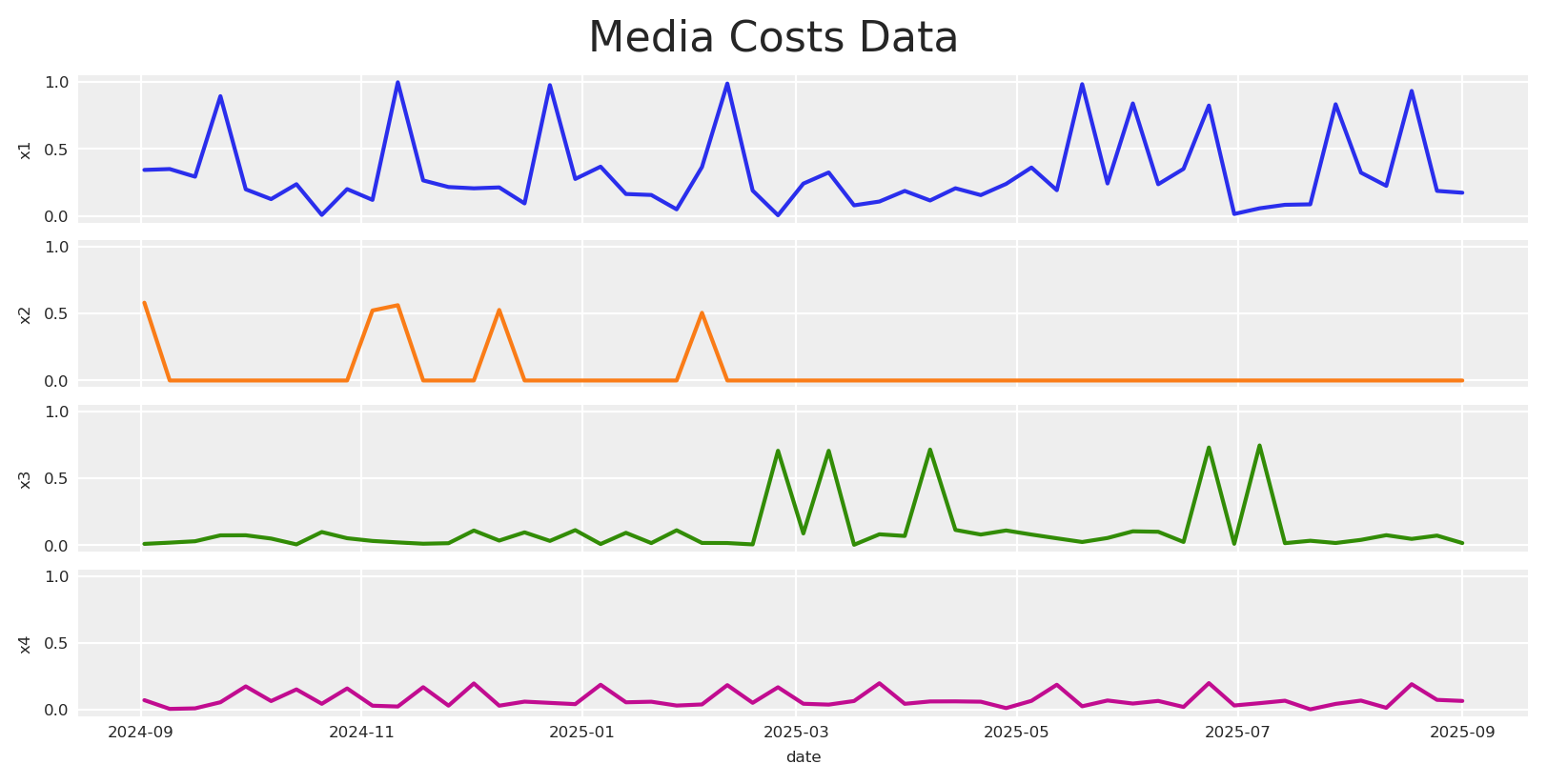
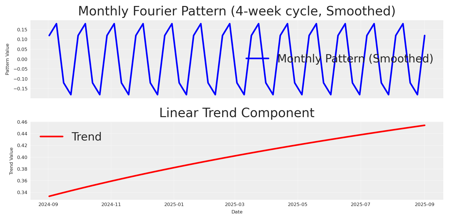
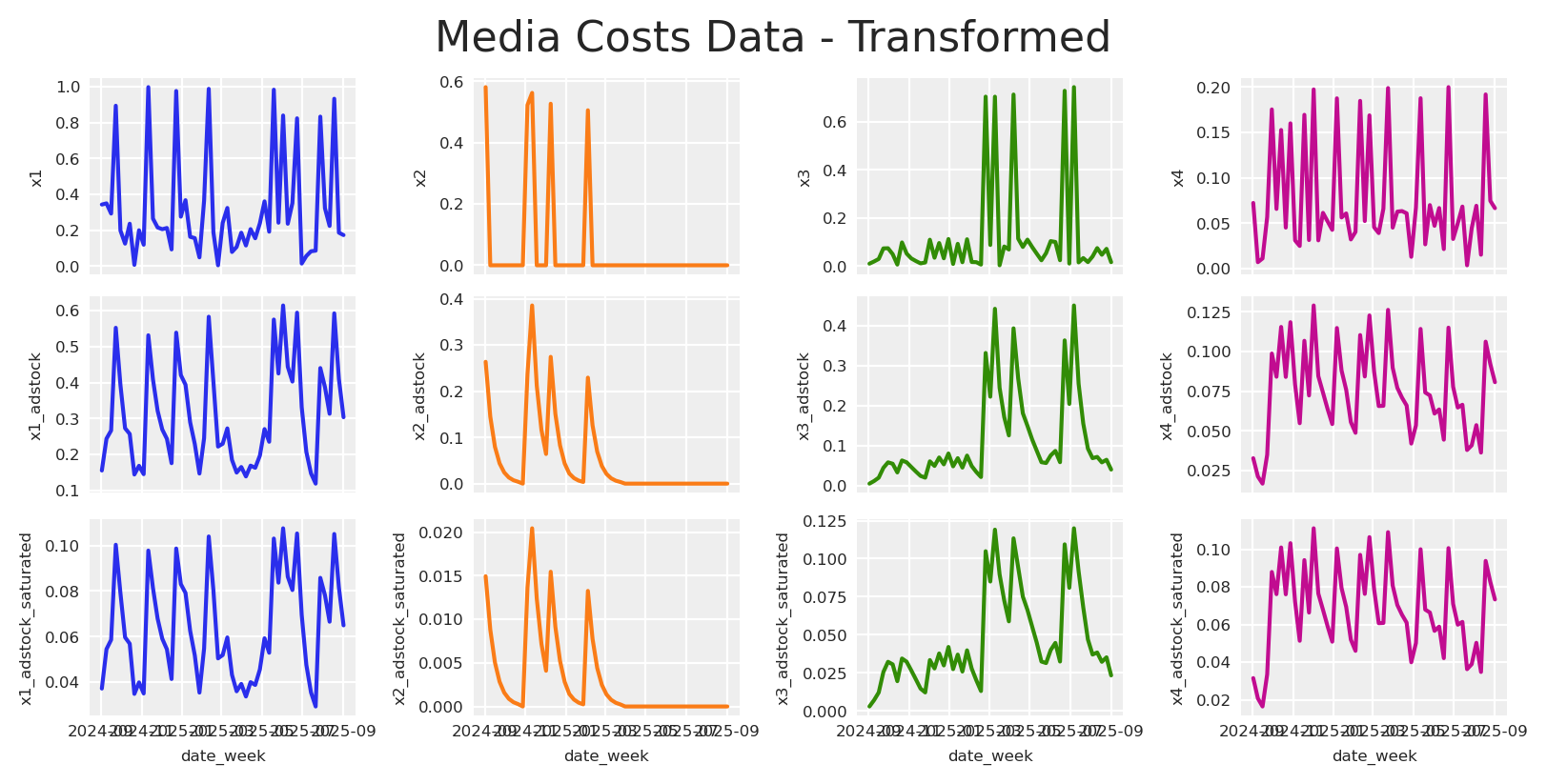
Modelos Bayesianos y optimización de riesgo para presupuestos de marketing, presentado en PyData Berlin 2025.
Autor/a
Carlos Trujillo
Fecha de publicación
20 de agosto de 2025
📘 Introducción
Este artículo explora cómo el Modelado Bayesiano de Mezcla de Medios (MMM) representa la incertidumbre y cómo podemos optimizar decisiones de presupuesto bajo riesgo. Construimos una vista generativa de la respuesta de medios (arrastre vía adstock, rendimientos decrecientes vía saturación, tendencia y estacionalidad) y usamos distribuciones predictivas posteriores completas para comparar asignaciones no solo por resultados esperados sino también por dispersión y riesgo de cola.
Este material acompaña mi charla en PyData Berlin 2025, donde discuto optimización práctica sensible al riesgo para MMM: ir más allá de planes que solo consideran la media hacia objetivos que incorporan explícitamente la incertidumbre—y cómo comunicar estas compensaciones a los stakeholders.
📦 Importar librerías
Código
import warningswarnings.filterwarnings("ignore", category=UserWarning)from pymc_marketing.mmm.builders.yaml import build_mmm_from_yamlfrom pymc_marketing.mmm import GeometricAdstock, MichaelisMentenSaturationfrom pymc_marketing.mmm.budget_optimizer import optimizer_xarray_builderfrom pymc_marketing.mmm.multidimensional import ( MultiDimensionalBudgetOptimizerWrapper,)from pymc_extras.prior import Priorfrom pymc_marketing.mmm import utility as utfrom scipy import ndimageimport arviz as azimport matplotlib.pyplot as pltimport seaborn as snsimport numpy as npimport pandas as pdimport xarray as xr
⚙️ Configuración del notebook
Código
az.style.use("arviz-darkgrid")plt.rcParams["figure.figsize"] = [8, 4]plt.rcParams["figure.dpi"] =100plt.rcParams["axes.labelsize"] =6plt.rcParams["xtick.labelsize"] =6plt.rcParams["ytick.labelsize"] =6plt.rcParams.update({"figure.constrained_layout.use": True})%load_ext autoreload%autoreload 2seed: int=sum(map(ord, "pydata_berlin_2025"))rng: np.random.Generator = np.random.default_rng(seed=seed)default_figsize = (8, 4) # repeat to use later
y_t es el resultado observado (por ejemplo, instalaciones de app o ingresos) en el tiempo t
\beta_0 es el intercepto base
f(x_{c,t}; \theta_c) es la función de respuesta de medios para el canal c con gasto x_{c,t} y parámetros \theta_c.
\text{trend}_t captura patrones de crecimiento o declive a largo plazo
\text{seasonality}_t modela efectos periódicos (patrones semanales, mensuales)
\varepsilon_t representa la incertidumbre aleatoria—ruido irreducible de factores no observados, error de medición y aleatoriedad inherente que persiste incluso con conocimiento perfecto de todos los parámetros
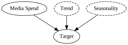
No consideramos interacciones; el DAG causal se ve así:
La configuración YAML codifica un MMM completamente Bayesiano con priors sobre la mecánica de respuesta central y la estructura temporal. Para detalles del modelo y ejemplos prácticos, consulta la Galería de ejemplos y el API de PyMC‑Marketing.
Aquí dividimos los datos en conjuntos de entrenamiento y prueba. No para evaluar el ajuste; en su lugar, usamos el conjunto de prueba para comparar los resultados de la optimización, verificando si será “mejor” en las recomendaciones de presupuesto que el plan actual/vigente.
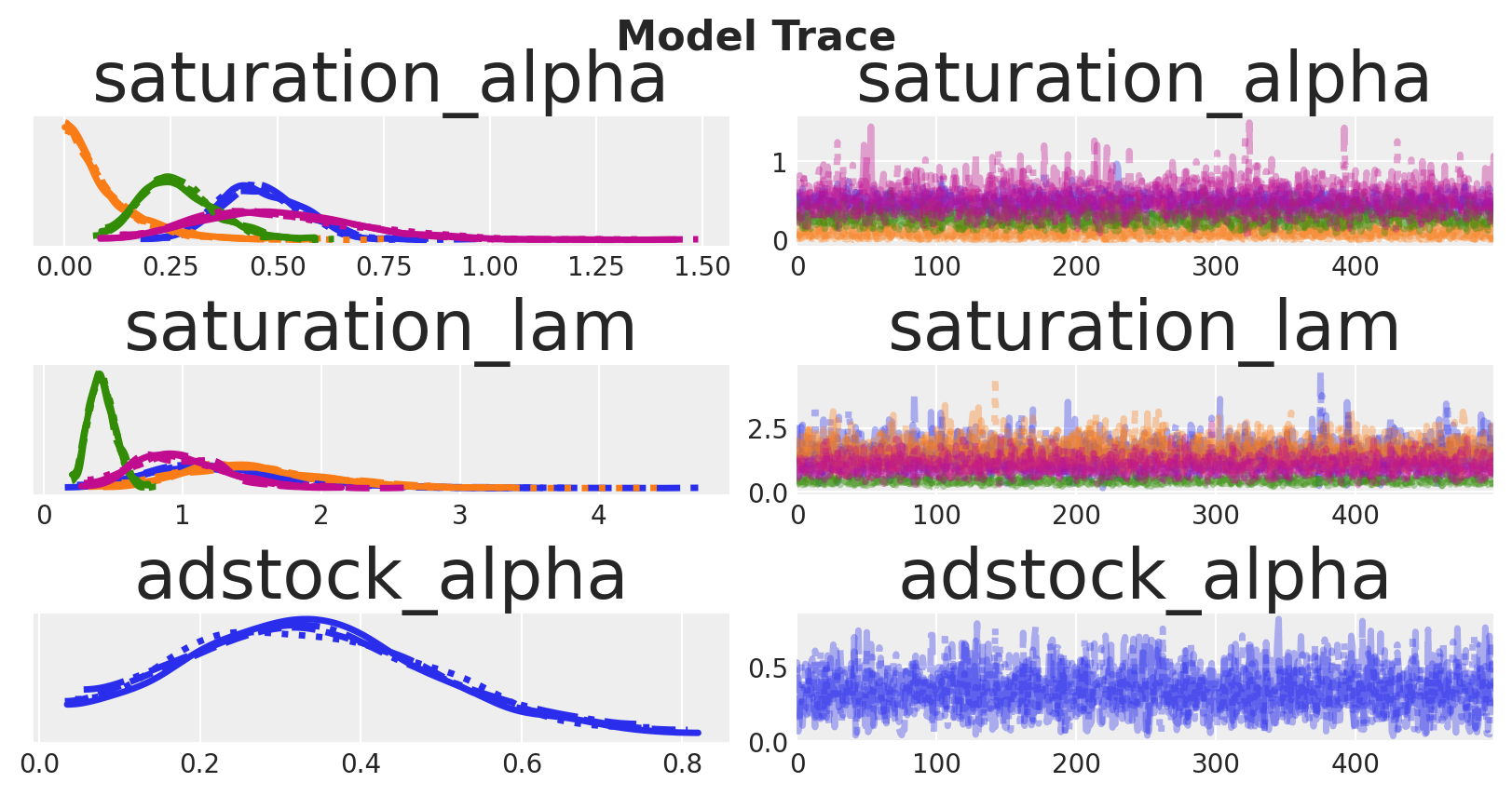
Como era de esperarse, algunos parámetros están bien identificados mientras otros permanecen inciertos.
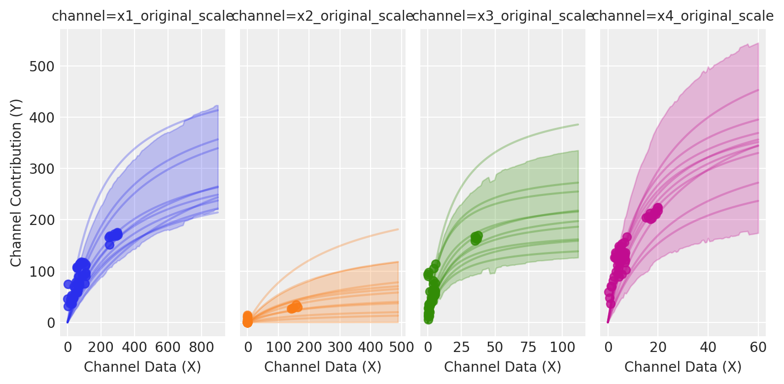
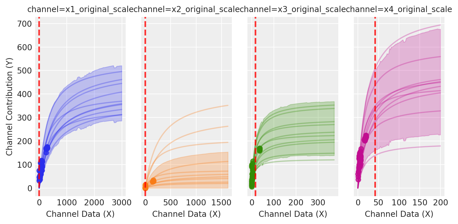
Muestrear curvas de saturación del posterior nos ayuda a visualizar la incertidumbre de parámetros como bandas alrededor de la respuesta de cada canal. Bandas anchas indican rendimientos marginales pobremente identificados; asignar en esas regiones incrementa la varianza del resultado porque pequeños cambios en los parámetros causan grandes cambios en la respuesta.
La imagen es clara: canales como X1 y X3 exhiben más variación entre niveles de gasto, permitiendo que el modelo aprenda sus parámetros con mayor precisión. Canales como X2 y X4 tienen un gasto relativamente constante con menos variación, por lo que sus parámetros se estiman con mayor incertidumbre.
🎲 Entendiendo la incertidumbre
En un MMM Bayesiano modelamos explícitamente dos formas de incertidumbre que se combinan en pronósticos y en decisiones de presupuesto:
Incertidumbre aleatoria: aleatoriedad en los resultados condicionada a parámetros fijos. En la simulación, esto es epsilon. Formalmente, si los parámetros son \theta, la incertidumbre aleatoria es la dispersión de p(y\mid x,\theta) una vez que modelamos la verosimilitud como \mathcal{N}(0, \sigma^2). En nuestro modelo, el parámetro \sigma captura explícitamente la incertidumbre aleatoria: cuantifica la cantidad de variabilidad del resultado que persiste incluso si todos los parámetros estructurales \theta fueran conocidos con exactitud. Representa la imprevisibilidad inherente debido a micro-variaciones no observadas, choques de demanda o ruido de registro. Incluso con datos infinitos, la incertidumbre aleatoria persiste.
Incertidumbre epistémica: incertidumbre sobre los parámetros y las funciones latentes debido a datos limitados o poco informativos. Esta es la dispersión del posterior p(\theta\mid \text{data}). Se reduce con más datos, mejores priors o mayor variación experimental. En nuestro modelo incluye la memoria de arrastre (adstock \alpha), la curvatura de saturación y saturación a la mitad (Michaelis–Menten \alpha,\lambda), pendientes de tendencia y pesos de Fourier estacionales.
Por qué esta separación importa para la planificación:
Distribución del resultado bajo un plan. Para un plan de asignación dado b sobre canales y tiempo, la predictiva posterior es
p\big(Y(b)\mid \text{data}\big) = \int p\big(Y(b)\mid \theta\big)\, p(\theta\mid \text{data})\, d\theta,
que mezcla variabilidad aleatoria (el término interno) y variabilidad epistémica (integración sobre \theta). Nuestro estimador de Monte Carlo muestrea \theta^{(s)} del posterior, simula arrastre y saturación bajo b, y extrae resultados predictivos.
Ejemplo: curvatura conocida vs desconocida. Supongamos que la saturación de un canal está bien aprendida alrededor de los gastos históricos pero no más allá. Dos planes con el mismo gasto total difieren en riesgo:
El plan A se concentra alrededor de la moda histórica (baja incertidumbre epistémica), produciendo una distribución predictiva estrecha.
El plan B se extiende más allá de los gastos observados (alta incertidumbre epistémica), produciendo una distribución más amplia y colas de pérdida más pesadas si la curva se aplana antes de lo esperado.
Durante la optimización, nos enfocamos en el segundo componente —incertidumbre epistémica— y podemos elegir cuánta confianza requerimos alrededor de ella. Una vez que elegimos una asignación, entonces incorporamos la incertidumbre aleatoria para cuantificar la distribución total de respuesta, si así lo deseamos.
🧭 Optimización
Pensemos en nuestro modelo y sus resultados, comenzando con la distribución predictiva posterior:
p\big(Y(b)\mid \text{data}\big) = \int p\big(Y(b)\mid \theta\big)\, p(\theta\mid \text{data})\, d\theta
Como puedes ver, la distribución predictiva posterior incorpora tanto incertidumbre aleatoria como epistémica, lo que significa que el problema de optimización se reduce a elegir una asignación b que optimice un resumen escalar de esta distribución.
Formalmente, sea b \in \mathbb{R}^C una asignación factible (por ejemplo, presupuestos por canal) con restricciones
\sum_{c=1}^C b_c = B, \qquad \underline{b}_c \leq b_c \leq \overline{b}_c.
Para cada asignación candidata b, obtenemos draws de Monte Carlo de la distribución predictiva posterior:
\{Y^{(s)}(b)\}_{s=1}^S \sim p(Y \mid \mathrm{do}(X=b), \mathcal{D}),
Luego se calcula un estadístico (por ejemplo, la media, un cuantil, una puntuación ajustada por riesgo, o el puntaje de concentración media).
\phi\!\left(\{Y^{(s)}(b)\}\right)
En consecuencia, el problema de optimización resuelto por SLSQP es simplemente
\min_{b \in \mathcal{B}} J(b), \qquad J(b) = f\!\left(\phi(\{Y^{(s)}(b)\})\right),
donde f se define de modo que el solucionador minimice el estadístico elegido de la distribución predictiva posterior.
Esta formulación es flexible: al cambiar \phi, podemos apuntar a criterios neutrales al riesgo o sensibles al riesgo o incluso heurísticos, mientras siempre fundamentamos la decisión en la distribución predictiva posterior.
💡 Notas sobre supuestos
¿Por qué decimos do=(X=b)?
Invariancia estructural: Las funciones de respuesta (tendencia, estacionalidad, adstock, saturación, enlace) son invariantes ante intervenciones b sobre el horizonte de optimización.
Sin confusión no medida: Condicionado a las covariables incluidas y controles temporales, no hay factores de confusión no medidos (especialmente variables en el tiempo) que afecten tanto el gasto como el resultado; se cumple el criterio de puerta trasera.
Usamos p\big(Y \mid \mathrm{do}(X=b), \mathcal{D}\big) como abreviatura para la predictiva posterior bajo estos supuestos. Cuando las asignaciones se alejan mucho del soporte, los resultados se vuelven extrapolativos y deben tratarse como análisis de sensibilidad en lugar de efectos identificados.
¿👀 Realmente Bayesiano?
Nuestro enfoque difiere de la “optimización Bayesiana” en el sentido de ML (que modela secuencialmente el objetivo con un sustituto y optimiza una función de adquisición). En contraste, ya tenemos el posterior completo p(\theta \mid \text{data}), que propagamos en la predictiva posterior p(Y(b)\mid \text{data}). La optimización entonces opera sobre un funcional escalar \phi de esta distribución. Esto puede verse como una compresión de la predictiva posterior en un resumen relevante para la decisión, pero no como una pérdida de información Bayesiana. La optimización permanece completamente Bayesiana porque el criterio depende enteramente de draws del posterior.
🛠️ Definir el optimizador
Inicializar el optimizador es directo: pasa el modelo y el rango de fechas.
Usaremos el conjunto de prueba para definir el presupuesto y el período de optimización para que podamos comparar la asignación resultante con nuestro plan actual.
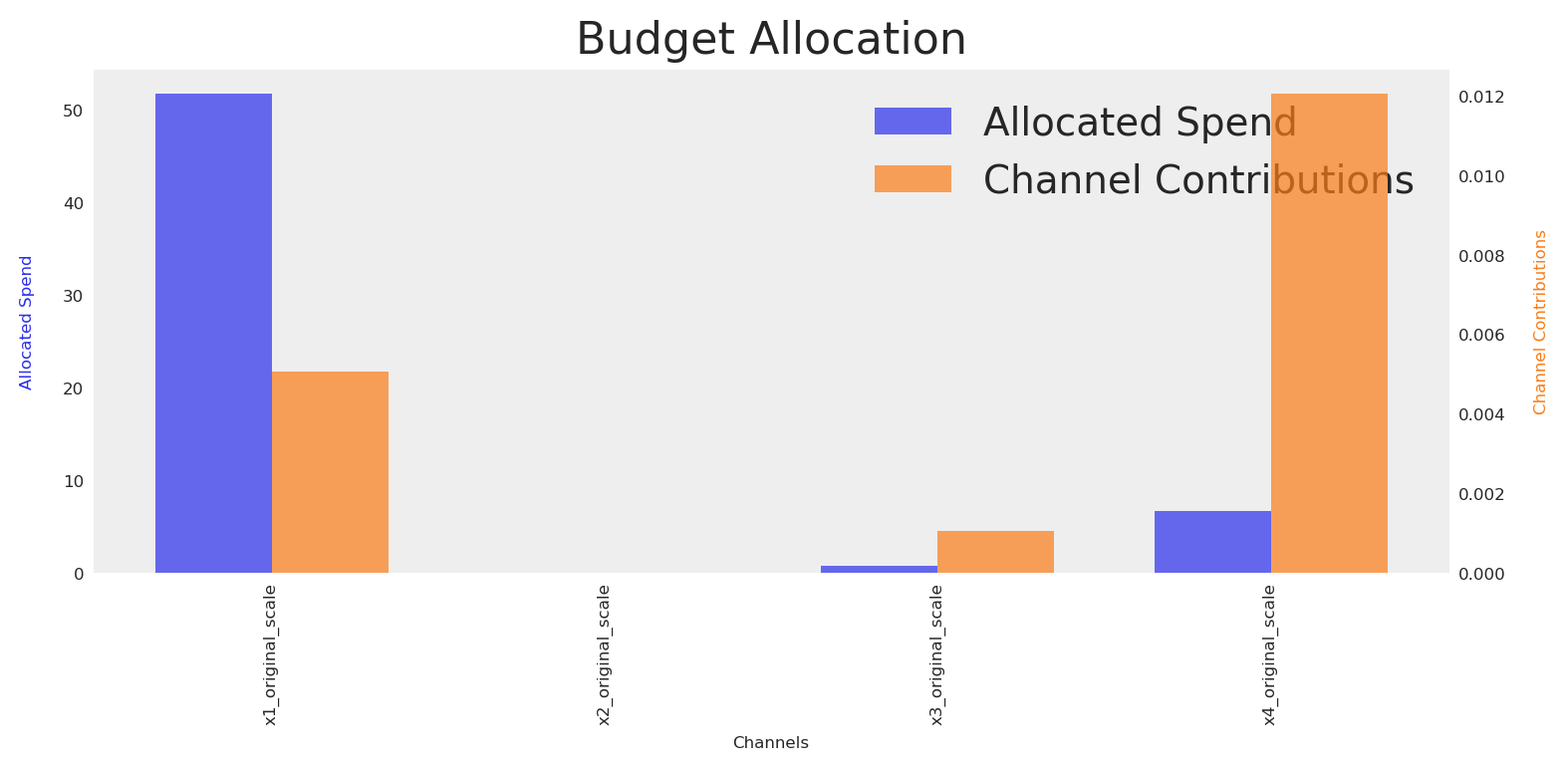
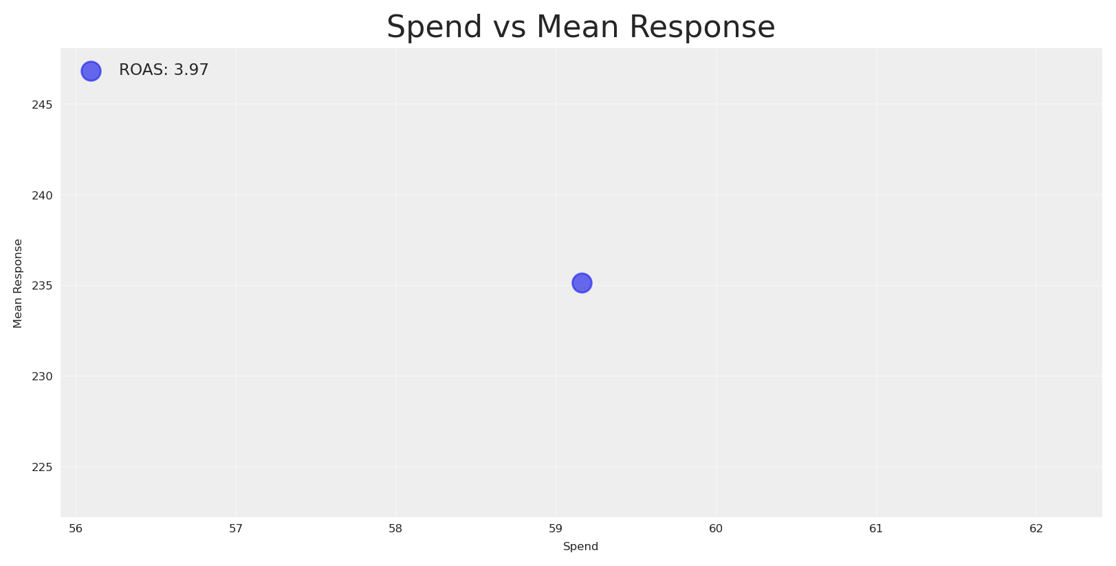
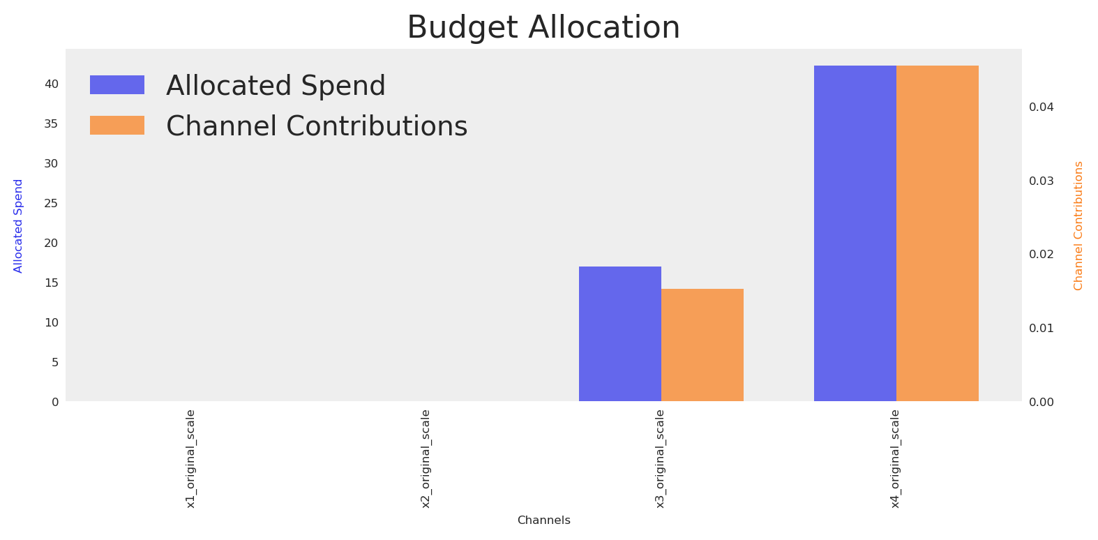
El plot.budget_allocation por defecto genera un gráfico de barras con asignación y respuesta por canal. Para ver los totales, podemos sumar y crear un gráfico de dispersión simple con una etiqueta para el ROAS.
Código
# Create scatterplot with spend and mean responsespend = initial_posterior_response.allocation.sum().valuesmean_response = initial_posterior_response.total_media_contribution_original_scale.mean(dim='sample').valuesinitial_roas = mean_response / spendplt.scatter(spend, mean_response, alpha=0.7, s=100, label=f"ROAS: {initial_roas:.2f}")plt.xlabel('Spend')plt.ylabel('Mean Response')plt.title('Spend vs Mean Response')plt.grid(True, alpha=0.3)plt.legend(fontsize='small', loc='upper left')plt.show()
Obtuvimos un ROAS de 3.9 para el plan inicial, que está por debajo de nuestro ROAS objetivo (digamos 8). Ahora podemos ejecutar una optimización estándar para responder la pregunta: ¿podemos reasignar para lograr una mayor respuesta dado el mismo presupuesto?
Budget allocation by channel:
  x1_original_scale: 0
  x2_original_scale: 0
  x3_original_scale: 16
  x4_original_scale: 42
Total Allocated Budget: 59
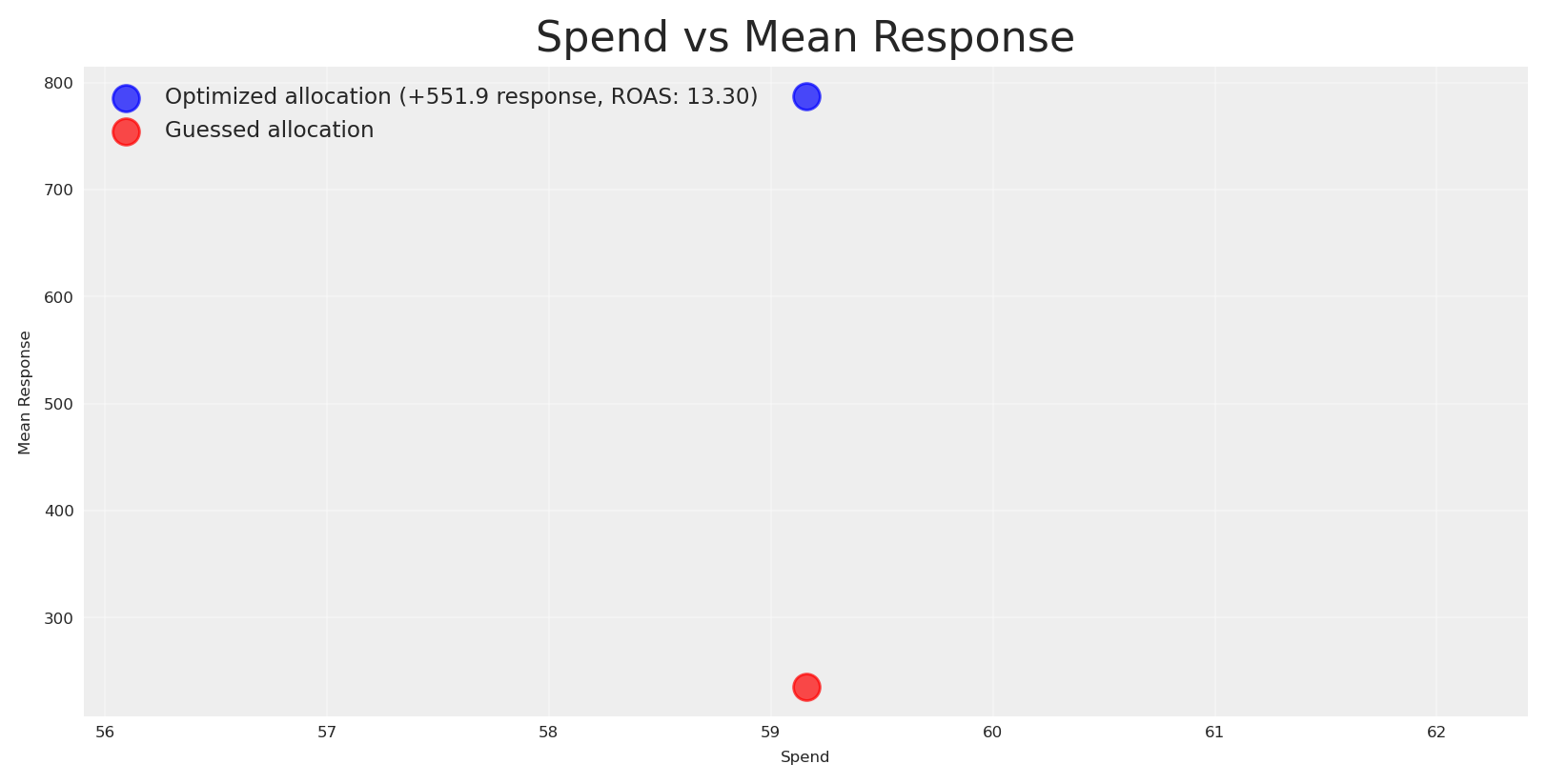
Sí, lo hacemos. Comparemos la respuesta optimizada contra el plan base.
Código
# Create scatterplot with spend and mean responsemean_response_v2 = naive_posterior_response.total_media_contribution_original_scale.mean(dim='sample').valuesroas_v2 = mean_response_v2 / spend# Calculate the delta in responseresponse_delta = mean_response_v2.sum() - mean_response.sum()plt.scatter(spend, mean_response_v2, alpha=0.7, s=100, color="blue", label=f"Optimized allocation (+{response_delta:.1f} response, ROAS: {roas_v2:.2f})")plt.scatter(spend, mean_response, alpha=0.7, s=100, color="red", label="Guessed allocation")plt.xlabel('Spend')plt.ylabel('Mean Response')plt.title('Spend vs Mean Response')plt.grid(True, alpha=0.3)plt.legend(fontsize='small', loc='upper left')plt.show()
La asignación optimizada es ~500 unidades mayor que la asignación estimada, y el nuevo ROAS estimado es 13, lo cual supera nuestras expectativas. En consecuencia, asumimos que obtendremos un ingreso Y estimado en los próximos N períodos y planificando contra este flujo de caja entrante recuperaremos la inversión.
¿El giro de la trama? Obtuvimos una respuesta menor, lo que significa un ROAS más bajo y tuvimos problemas financieros serios porque no tenemos suficiente efectivo para pagar a proveedores o servicios.
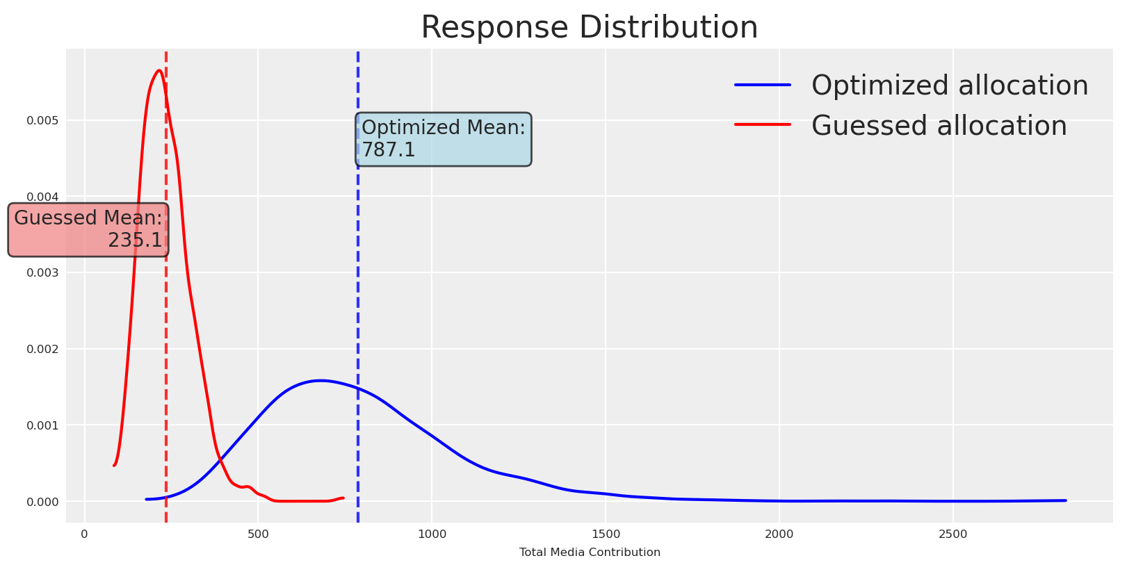
¿Por qué ocurre esto? Maximizar la respuesta media es neutral al riesgo. A menudo reasigna el presupuesto hacia regiones con potenciales altos retornos aunque estén débilmente identificadas, aumentando la dispersión de los resultados. Esto es racional cuando los stakeholders son indiferentes al riesgo. Sin embargo, ese no es el caso para todas las empresas. A veces nuestros stakeholders necesitan saber qué tan seguros estamos sobre los resultados esperados.
Al inspeccionar muestras predictivas posteriores bajo cada asignación, podemos cuantificar la incertidumbre y responder esta pregunta, basándonos en la comprensión actual del modelo.
Grafiquemos las distribuciones de respuesta para ambas asignaciones, la base y la optimizada.
Código
fig, ax = plt.subplots()# Get the valuesoptimized_values = naive_posterior_response.total_media_contribution_original_scale.valuesguessed_values = initial_posterior_response.total_media_contribution_original_scale.values# Plot distributionsaz.plot_dist( optimized_values, color="blue", label="Optimized allocation", ax=ax,)az.plot_dist( guessed_values, color="red", label="Guessed allocation", ax=ax,)# Calculate meansoptimized_mean = optimized_values.mean()guessed_mean = guessed_values.mean()# Add vertical lines for meansax.axvline(optimized_mean, color="blue", linestyle="--", alpha=0.8)ax.axvline(guessed_mean, color="red", linestyle="--", alpha=0.8)# Add text boxes with mean valuesax.text(optimized_mean +10, ax.get_ylim()[1] *0.8, f'Optimized Mean:\n{optimized_mean:.1f}', bbox=dict(boxstyle="round,pad=0.3", facecolor="lightblue", alpha=0.7), ha='left', va='center')ax.text(guessed_mean -10, ax.get_ylim()[1] *0.6, f'Guessed Mean:\n{guessed_mean:.1f}', bbox=dict(boxstyle="round,pad=0.3", facecolor="lightcoral", alpha=0.7), ha='right', va='center')plt.title("Response Distribution")plt.xlabel("Total Media Contribution")plt.legend()plt.show()
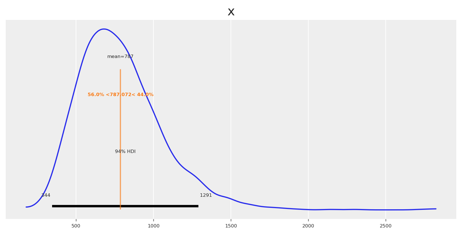
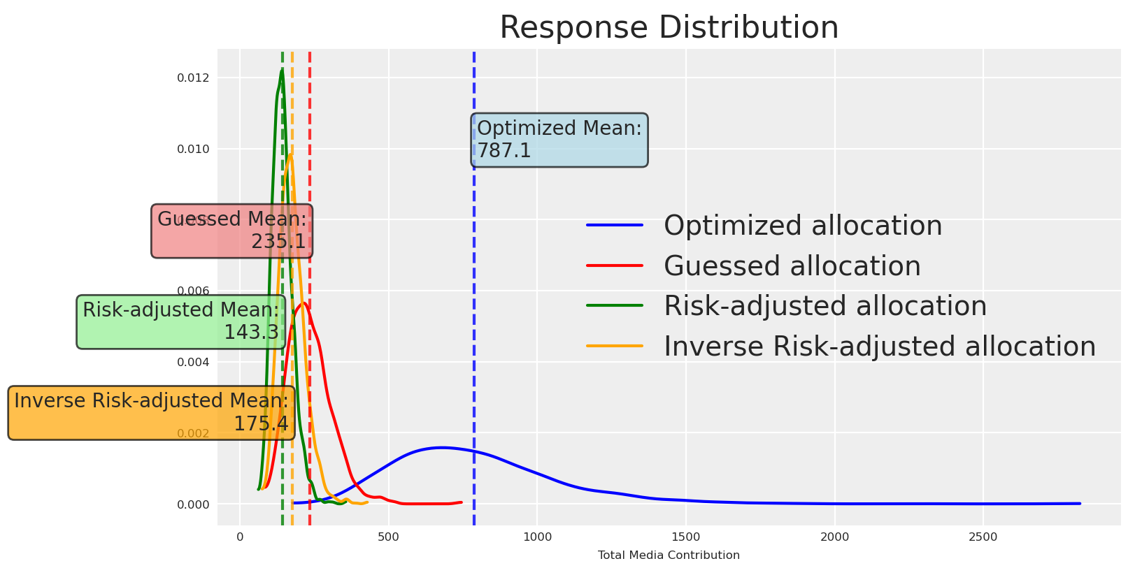
Como era de esperarse, las medias difieren (optimizamos para incrementarla), y lo mismo ocurre con la certeza alrededor de la media. Como ejercicio, observemos qué tan probable es obtener una respuesta mayor y menor que la media.
Esto aclara todo ahora; las probabilidades de obtener algo mayor o igual que la media eran del 43% pero las probabilidades de obtener algo menor que la media eran del 56%. No es sorpresa que obtuviéramos una respuesta menor y un ROAS más bajo.
💡 Primera conclusión
Comparar distribuciones completas hace el riesgo transparente: la amplitud cuantifica la confiabilidad del pronóstico, la asimetría revela la asimetría entre oportunidad y riesgo, y las superposiciones muestran indistinguibilidad práctica.
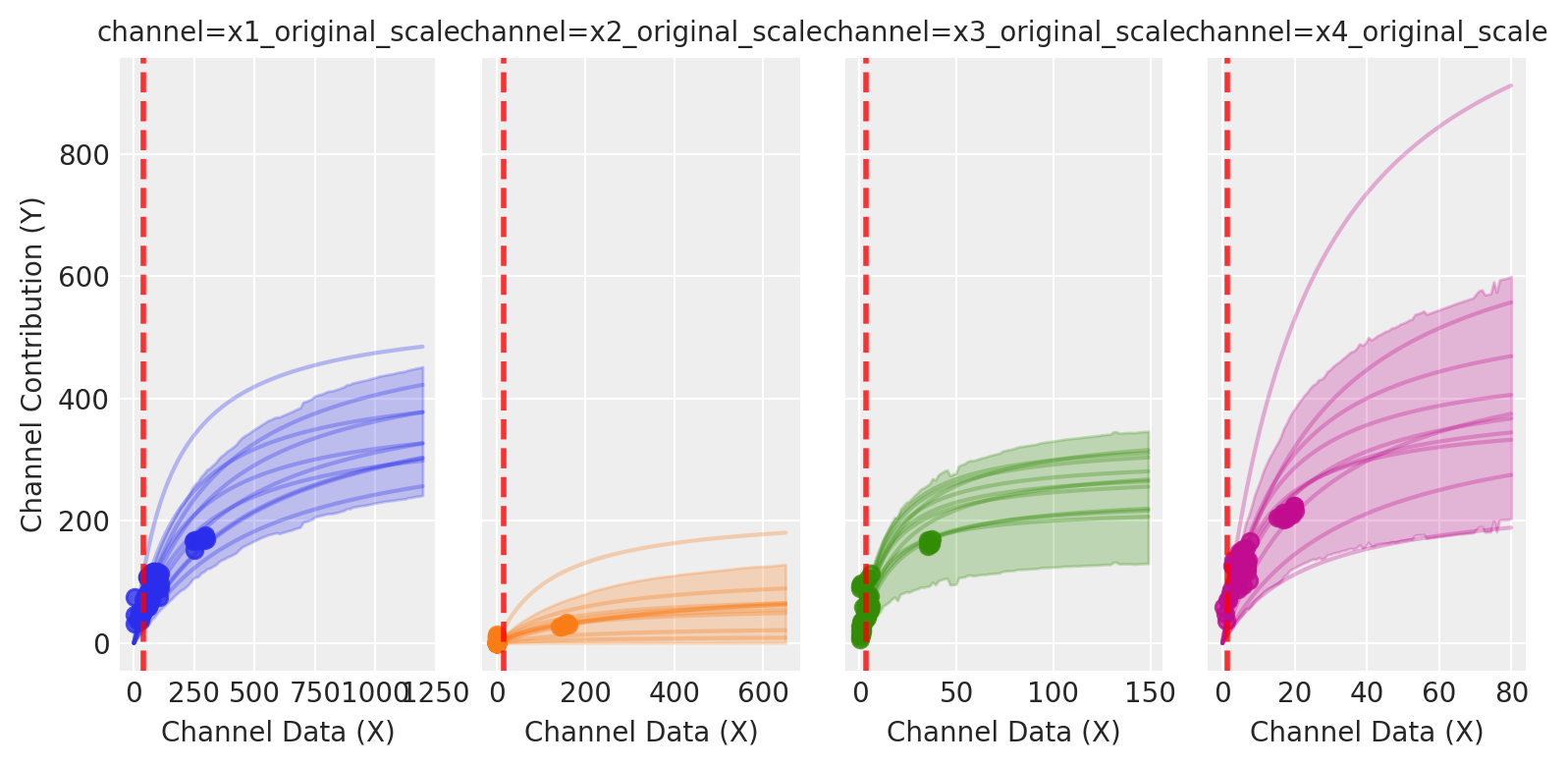
¿De dónde viene este riesgo? La nueva asignación es más riesgosa, pero ¿por qué? Veamos cada nivel de gasto en relación con su curva de saturación.
Las líneas verticales se ubican en la asignación de gasto dada para cada canal. Para canales como x4, el modelo tiene pocas observaciones en esos niveles de gasto, por lo que las bandas posteriores son amplias y la distribución de respuesta inducida es difusa. La optimización sensible al riesgo tiende a atraer el gasto hacia regiones bien identificadas (a menudo cerca del punto de inflexión), intercambiando una pequeña disminución de la media por una gran reducción en la varianza.
¿Podríamos entender esto de antemano? Y si es así, ¿preferiríamos un tipo diferente de asignación? ¿Cuál nos acerca a nuestro objetivo de una forma más segura? -Una distribución más estrecha con una media ligeramente menor puede ser preferible cuando el riesgo de déficit es costoso-.
La respuesta corta es definitivamente. Creemos ahora un nuevo proceso de optimización que sea sensible al riesgo.
⚖️ Métricas de riesgo consistentes con PyMC-Marketing
Aquí usaremos una aproximación heurística, el puntaje de concentración media (mean tightness score) implementado en la librería PyMC-Marketing. Este puntaje combina la media con una penalización por dispersión en las colas.
🎯 Puntaje de concentración media (Mean Tightness Score)
Código
ut.mean_tightness_score?
Alpha codifica tu perfil de riesgo (rango 0-1); las asignaciones con medias más altas, incluso si tienen gran dispersión, puntúan mejor cuando tu alpha es alto. Cuando tu alpha es bajo, las asignaciones con medias más bajas pero baja dispersión puntúan mejor.
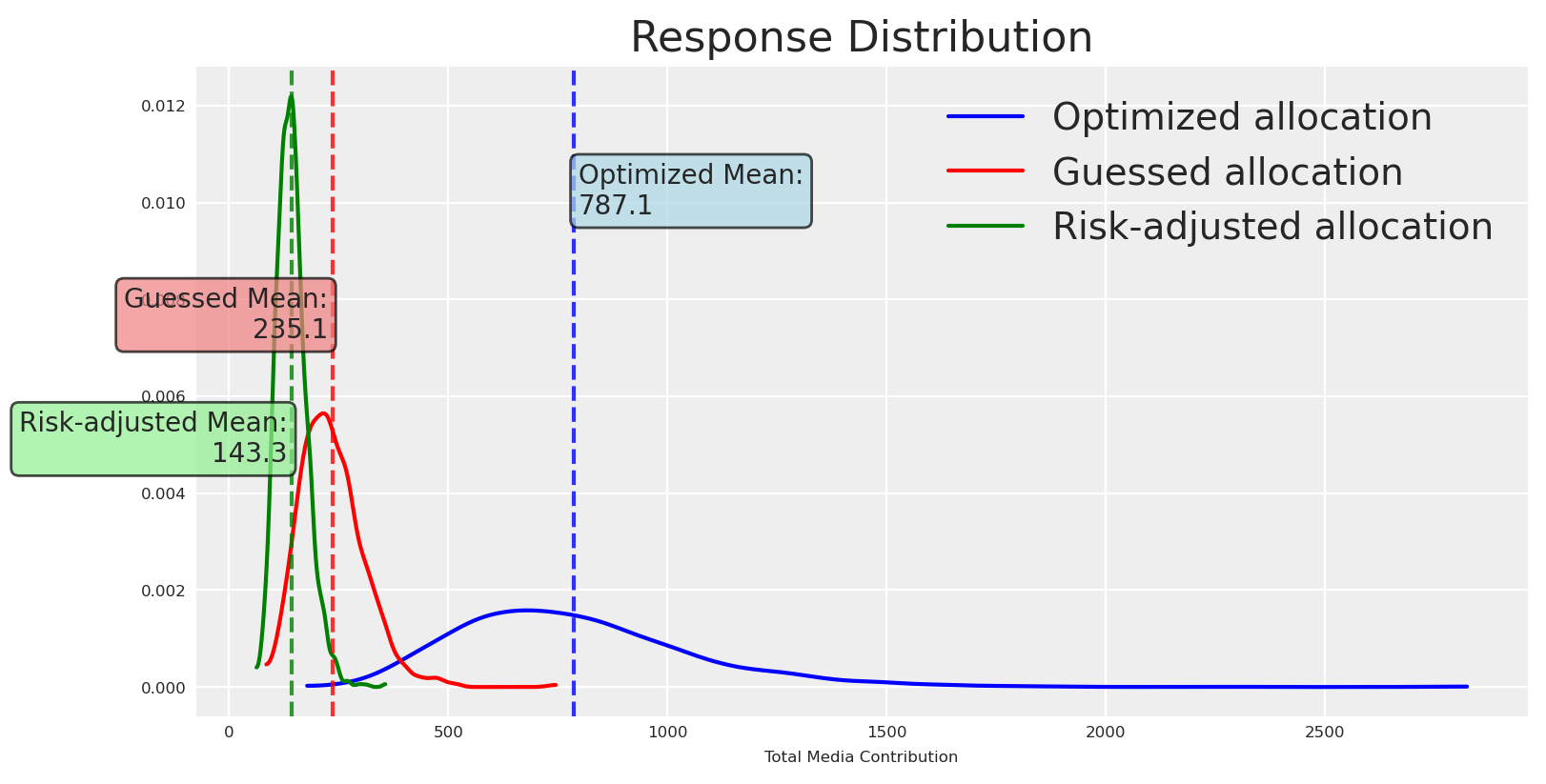
Estamos usando un alpha más bajo en el ejemplo; como era de esperarse, las recomendaciones para cada canal se encuentran en regiones bien conocidas.
Esto lo deja claro: ganamos mucha más certeza—una distribución de respuesta adversa al riesgo (de menor varianza). Puede que estés pensando que operar en regiones conocidas tiende a reducir la media. ¿Quieres saber por qué?
Las curvas de respuesta posteriores tienden a ser más seguras en el origen porque dos fuentes de incertidumbre se minimizan ahí: estructuralmente, sabemos que cero gasto produce cero efecto incremental, y empíricamente, la región de menor gasto suele estar bien respaldada en los datos históricos. A medida que el gasto aumenta, especialmente más allá de los niveles históricamente observados, la incertidumbre epistémica sobre los parámetros de saturación y curvatura domina, ensanchando los intervalos creíbles.
¿Eso significa que estamos condenados a valores más bajos si queremos certeza? Para nada; podemos cambiar la utilidad para preferir opciones más arriesgadas 🔥.
Ejecutemos una asignación más orientada al riesgo 👀
Budget allocation by channel:
  x1_original_scale: 50
  x2_original_scale: 3
  x3_original_scale: 3
  x4_original_scale: 2
Total Allocated Budget: 59
Invertir la preferencia de concentración (parámetro alpha) induce comportamiento de búsqueda de riesgo, moviendo las asignaciones hacia regiones de mayor varianza y alto potencial alcista.
Ahora elegimos una asignación que es menos segura pero con mayor potencial alcista que la base. Grafiquemos las distribuciones de respuesta.
💡 Segunda conclusión
Descubre tus preferencias de riesgo y ajusta tu función objetivo para reflejarlas. No necesitas comprometerte con una sola función o enfoque; puedes crear una personalizada que se adapte a tus necesidades.
Genial, la nueva asignación es más riesgosa y la media es más alta (aún con menos incertidumbre que la asignación neutral al riesgo). Podemos ir más allá de lo visual y cuantificar esto.
Como todas son distribuciones posteriores, podemos verificar la densidad que tiene cada distribución de respuesta en su respectiva media. Usaremos estimación de densidad por kernel (KDE). Este valor, denotado \hat{f}(\mu), representa la altura estimada de la función de densidad de probabilidad en la media. Es importante destacar que esto no es en sí una probabilidad sino una densidad, con unidades de “1 sobre las unidades de la variable.” Valores más altos de \hat{f}(\mu) indican que la distribución tiene un pico pronunciado alrededor de la media, reflejando mayor certeza de que los draws del posterior se encuentren cerca del valor central. Por el contrario, valores más bajos corresponden a posteriores más planas y difusas, indicando mayor incertidumbre.
Revisemos la densidad en la media para cada asignación.
Código
from scipy.stats import gaussian_kdedef kde_density_at_point(x, x0):"""Gaussian KDE density estimate at x0 using Scott's rule bandwidth.""" kde = gaussian_kde(x) # Scott's rule by defaultreturnfloat(kde.evaluate([x0])[0])optimized_density = kde_density_at_point(optimized_values, optimized_mean)guessed_density = kde_density_at_point(guessed_values, guessed_mean)risk_adjusted_density = kde_density_at_point(optimized_risk_values, risk_adjusted_mean)inverse_risk_adjusted_density = kde_density_at_point(optimized_inverse_risk_values, inverse_risk_adjusted_mean)print(f"Optimized allocation response density at mean: {optimized_density:.3f}")print(f"Guessed allocation response density at mean: {guessed_density:.3f}")print(f"Risk-adjusted allocation response density at mean: {risk_adjusted_density:.3f}")print(f"Inverse Risk-adjusted allocation response density at mean: {inverse_risk_adjusted_density:.3f}")
Optimized allocation response density at mean: 0.001
Guessed allocation response density at mean: 0.005
Risk-adjusted allocation response density at mean: 0.012
Inverse Risk-adjusted allocation response density at mean: 0.010
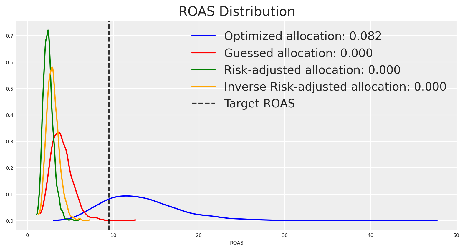
Las estimaciones de densidad cuentan la misma historia que los gráficos. ¿Cómo podemos usar esto para tomar acciones? Por ejemplo, supongamos que queremos alcanzar un ROAS objetivo de 9.5; entonces podemos verificar la densidad de la distribución de ROAS en 9.5 para cada distribución de respuesta dada su respectiva estrategia de asignación.
Si queremos alcanzar un ROAS objetivo de 9.5, la asignación optimizada neutral al riesgo es la más segura, seguida por la asignación inversa ajustada por riesgo.
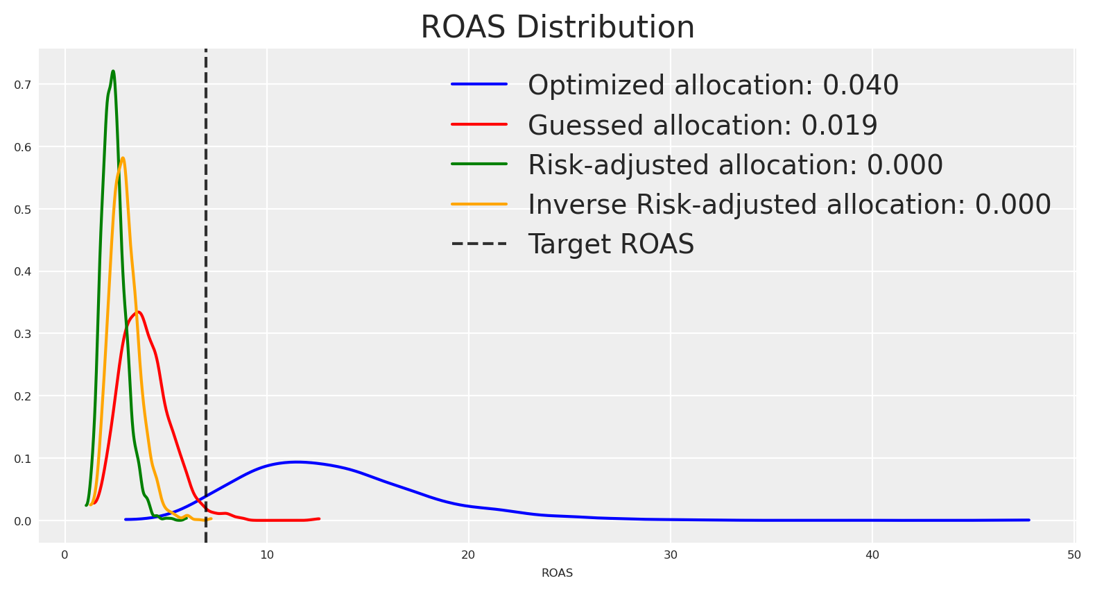
Si en cambio nuestro ROAS objetivo es 7, la asignación inversa ajustada por riesgo concentra más densidad alrededor de ese valor, y la asignación optimizada neutral al riesgo tiene menos densidad alrededor.
Bajo este paradigma, puedes definir un objetivo estimado y seleccionar una asignación que maximice la probabilidad de alcanzarlo. Una forma es crear una función que reduzca la varianza con respecto al objetivo, favoreciendo distribuciones más estrechas con densidad cerca del objetivo.
Creemos esta función de utilidad personalizada, y veamos cómo funciona.
Código
import pytensor.tensor as ptimport pymc_marketing.mmm.utility as utdef target_hit_probability(target, num_periods):""" Target hit probability utility function. Minimizing the mean squared error between predicted ROAS and the target Adding a variance penalty to encourage tighter distributions. Parameters ---------- target : float The target ROAS value to optimize towards num_periods : int Number of time periods for the budget allocation Returns ------- callable A utility function that can be used with the budget optimizer. Returns negative objective (since optimizer minimizes). """def _function(samples, budgets): roas_samples = samples / (pt.sum(budgets) * num_periods)# Use mean squared error from target, which provides smoother gradients mse_from_target = pt.mean((roas_samples - target) **2)# Add penalty for variance to encourage tighter distributions around target variance_penalty = pt.var(roas_samples)# Combine MSE and variance penalty with weighting# Higher variance penalty encourages narrower distributions total_objective = mse_from_target +0.1* variance_penaltyreturn-total_objectivereturn _function_roas_target =10custom_utility_budget_allocation, custom_utility_optimizer_result, callback_results = ( optimizable_model.optimize_budget( budget=time_unit_budget, utility_function=target_hit_probability(_roas_target, num_periods), callback=True, minimize_kwargs={"options": {"maxiter": 2_000}}, ))custom_utility_posterior_response = optimizable_model.sample_response_distribution( allocation_strategy=custom_utility_budget_allocation, include_carryover=True, include_last_observations=False, additional_var_names=["y_original_scale"])# Print budget allocation by channelprint("Budget allocation by channel:")for channel in channels:print(f" {channel}: {custom_utility_posterior_response.allocation.sel(channel=channel).astype(int).sum():,}" )print(f"Total Allocated Budget: {np.sum(custom_utility_posterior_response.allocation.to_numpy()):,.0f}")
Budget allocation by channel:
  x1_original_scale: 23
  x2_original_scale: 0
  x3_original_scale: 23
  x4_original_scale: 12
Total Allocated Budget: 59
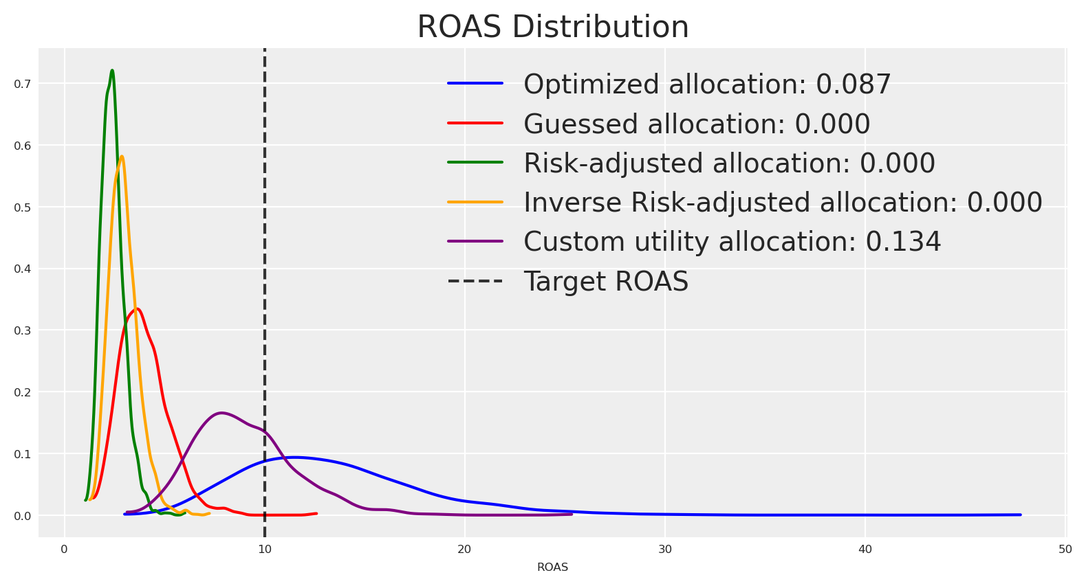
La asignación es similar a las observadas anteriormente. Grafiquemos las distribuciones de ROAS.
Genial 🙌🏻 La asignación optimizada inicial, que era neutral al riesgo, tenía inicialmente la mayor densidad alrededor del ROAS objetivo, pero la densidad alrededor no era suficientemente alta; la nueva asignación proporciona una respuesta más segura alrededor del objetivo, porque la función objetivo fue construida para eso.
💡 Hallazgo clave
Aquí tenemos una función de utilidad personalizada que nos permite optimizar para un ROAS objetivo. Sin embargo, puedes crear otras utilidades y usarlas como objetivos. También puedes introducir restricciones sensibles al riesgo—encima de tus restricciones de negocio.
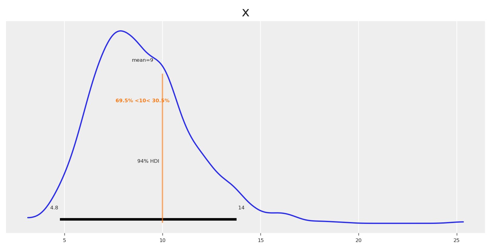
Observemos nuestro posterior final alrededor del ROAS objetivo.
Podríamos decir: la probabilidad de lograr ROAS ≥ 10 con esta asignación es del 31%, y ROAS < 10 es del 69%. Si necesitamos más certeza, podemos hacer la optimización más adversa al riesgo.
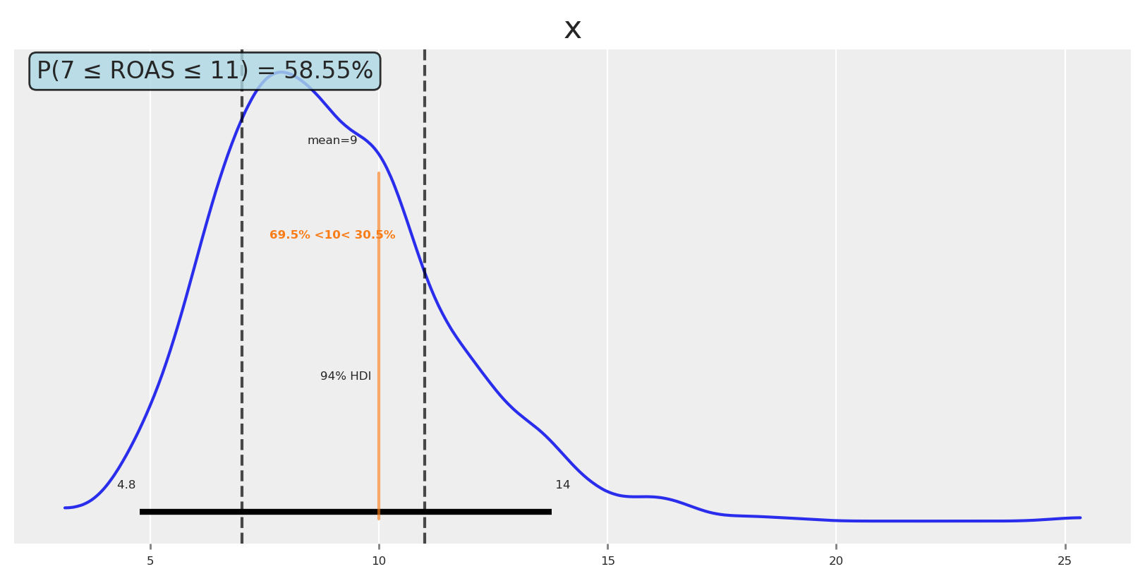
Ahora, si quieres pensar realmente de forma Bayesiana, puedes definir una región de equivalencia práctica, y verificar la probabilidad de que el ROAS esté en esa región. Por ejemplo, puedes preguntarte: ¿Haría algo diferente si el ROAS es 7, 9 u 11? Si la respuesta es no, entonces encontraste tu ROPE.
Digamos que queremos saber la probabilidad de que el ROAS esté entre 7 y 11.
Código
# Calculate probability of ROAS being between 7 and 9prob_7_to_11 = np.mean((custom_utility_roas >=7) & (custom_utility_roas <=11))# Plot posterior with reference values and regionfig, ax = plt.subplots()az.plot_posterior( custom_utility_roas, ref_val=_roas_target, ax=ax)# Add vertical lines for the region of interestax.axvline(7, color="black", linestyle="--", alpha=0.7, label="ROAS = 7")ax.axvline(11, color="black", linestyle="--", alpha=0.7, label="ROAS = 11")# Add text box with probabilityax.text(0.02, 0.98, f'P(7 ≤ ROAS ≤ 11) = {prob_7_to_11:.2%}', transform=ax.transAxes, bbox=dict(boxstyle="round,pad=0.3", facecolor="lightblue", alpha=0.8), ha='left', va='top', fontsize=12)plt.show()
💡 Hallazgo clave
Puedes definir una región de equivalencia práctica (ROPE), para ser más preciso en tu toma de decisiones. Esta es una forma bastante natural de pensar un problema, y alivia la carga del tomador de decisiones de comprometerse con un solo número. Al final del día, no necesitamos ser 99.999% precisos alrededor de cada respuesta o número; podemos ser 95% o 90% precisos y a veces eso es suficiente. Identifica si ese es tu caso, y piensa en consecuencia.
✅ Conclusiones sobre incertidumbre
Trata la incertidumbre como ciudadana de primera clase: Optimiza sobre la distribución predictiva posterior completa, no sobre estimaciones puntuales. Compara planes por sus distribuciones, no solo por las medias esperadas.
Comprende los tipos de incertidumbre: Aleatoria (ruido irreducible) vs epistémica (incertidumbre del modelo/parámetros que se puede reducir). Las decisiones de planificación principalmente desplazan el riesgo epistémico; siempre comunica ambos.
Encuentra tu apetito de riesgo: Pregunta a los stakeholders qué tan seguros debemos estar sobre los resultados reportados. ¿Qué cambia si son un poco más altos o más bajos?
Elige una utilidad alineada con tu apetito de riesgo: Trabajar con la media es neutral al riesgo; los cuantiles, TailDistance, CVaR o MTS son más sensibles al riesgo.
Comunica distribuciones, no números aislados: Muestra HDIs/cuantiles y probabilidades (por ejemplo, P(ROAS ≥ objetivo)). Es mejor entender el espectro completo de posibilidades que seguir números aislados y ser cortoplacista.
Define una región de equivalencia práctica (ROPE): Una vez que estés cómodo con la incertidumbre, experimenta con ROPEs y descubre cuánto podrías aligerar la respuesta estimada, y si harías algo diferente si esta cambia dentro de un rango de valores.
🚧 Limitaciones
Este enfoque representa la confianza del modelo, pero los modelos pueden estar muy seguros de una respuesta incorrecta. Siempre agrega conocimiento del negocio y salvaguardas para mantener las recomendaciones realistas.
Conclusión
Espero que este artículo haya sido útil para entender cómo usar modelos de mezcla de medios Bayesianos para optimizar tu gasto en medios. Entender la incertidumbre es una herramienta poderosa para tomar mejores decisiones, pero no es una solución mágica.
El ejemplo actual es sencillo; las aplicaciones en la vida real son más complejas y requieren modelos más sofisticados, funciones de riesgo y problemas de optimización complejos, donde las restricciones y el conocimiento del negocio son clave.
En PyMC Labs estamos construyendo herramientas para hacer este proceso más sencillo. Si te interesa aprender más, explora la Galería de ejemplos y el API de PyMC‑Marketing, nuestra documentación y blog.
Puedes obtener una consulta gratuita de 30 minutos con nuestro equipo para discutir tus necesidades específicas y cómo podemos ayudarte.
---title: "Bayesian Models and Risk Optimization"author: "Carlos Trujillo"date: "2025-08-20"description: "Bayesian models and risk optimization for marketing budgets, presented at PyData Berlin 2025."categories: [MMM, python, optimization, media mix modeling, bayesian, pymc, pydata, germany, berlin]image: "/images/bayesian_models_and_risk_optimization.jpg"image-alt: "Bayesian model risk optimization visualization for marketing budget allocation"jupyter: bayesian_models_and_risk_optimizationformat: html: code-fold: true code-tools: true code-overflow: wrap---# 📘 IntroductionThis article explores how Bayesian Media Mix Modeling (MMM) represents uncertainty and how we can optimize budget decisions under risk. We build a generative view of media response (carryover via adstock, diminishing returns via saturation, trend and seasonality) and use full posterior predictive distributions to compare allocations not only by expected outcomes but also by dispersion and tail risk.This material accompanies my PyData Berlin 2025 talk, where I discuss practical risk-aware optimization for MMM: moving beyond mean-only plans to objectives that explicitly incorporate uncertainty—and how to communicate these trade-offs to stakeholders.# 📦 Import libraries```{python}#| warning: falseimport warningswarnings.filterwarnings("ignore", category=UserWarning)from pymc_marketing.mmm.builders.yaml import build_mmm_from_yamlfrom pymc_marketing.mmm import GeometricAdstock, MichaelisMentenSaturationfrom pymc_marketing.mmm.budget_optimizer import optimizer_xarray_builderfrom pymc_marketing.mmm.multidimensional import ( MultiDimensionalBudgetOptimizerWrapper,)from pymc_extras.prior import Priorfrom pymc_marketing.mmm import utility as utfrom scipy import ndimageimport arviz as azimport matplotlib.pyplot as pltimport seaborn as snsimport numpy as npimport pandas as pdimport xarray as xr```# ⚙️ Notebook setup ```{python}#| warning: falseaz.style.use("arviz-darkgrid")plt.rcParams["figure.figsize"] = [8, 4]plt.rcParams["figure.dpi"] =100plt.rcParams["axes.labelsize"] =6plt.rcParams["xtick.labelsize"] =6plt.rcParams["ytick.labelsize"] =6plt.rcParams.update({"figure.constrained_layout.use": True})%load_ext autoreload%autoreload 2seed: int=sum(map(ord, "pydata_berlin_2025"))rng: np.random.Generator = np.random.default_rng(seed=seed)default_figsize = (8, 4) # repeat to use later```# 🧪 Data generation process We simulate outcomes as$$y_t = \beta_0 + \sum_{c} f(x_{c,t}; \theta_c) + \text{trend}_t + \text{seasonality}_t + \varepsilon_t$$where:- $y_t$ is the observed outcome (e.g., app installs or revenue) at time $t$- $\beta_0$ is the baseline intercept- $f(x_{c,t}; \theta_c)$ is the media response function for channel $c$ with spend $x_{c,t}$ and parameters $\theta_c$.- $\text{trend}_t$ captures long-term growth or decline patterns- $\text{seasonality}_t$ models periodic effects (weekly, monthly patterns)- $\varepsilon_t$ represents aleatoric uncertainty—irreducible noise from unobserved factors, measurement error, and inherent randomness that remains even with perfect knowledge of all parametersWe do not consider interactions; the causal DAG looks like this:```{python}#| warning: falseimport graphvizgraph = graphviz.Digraph()graph.node("Media Spend")graph.node("Trend", style="dashed")graph.node("Seasonality", style="dashed")graph.node("Target")graph.edge("Media Spend", "Target")graph.edge("Trend", "Target")graph.edge("Seasonality", "Target")graph```## 📆 Date rangeWe start by defining the date range.```{python}#| warning: false# date rangemin_date = pd.to_datetime("2024-09-01")max_date = pd.to_datetime("2025-09-01")df = pd.DataFrame( data={"date_week": pd.date_range(start=min_date, end=max_date, freq="W-MON")})n = df.shape[0]print(f"Number of observations: {n}")print("Date Range: {} to {}".format(df.date_week.min(), df.date_week.max()))```## 📣 Media data```{python}#| warning: false# media datascaler_x1 =300scaler_x2 =280scaler_x3 =50scaler_x4 =100y_scaler =1000# media datax1 = rng.uniform(low=0.0, high=1.0, size=n)df["x1"] = np.where(x1 >0.8, x1, x1 /2)x2 = rng.uniform(low=0.0, high=0.6, size=n)df["x2"] = np.where(x2 >0.5, x2, 0)x3 = rng.uniform(low=0.0, high=0.8, size=n)df["x3"] = np.where(x3 >0.7, x3, x3 /6)x4 = rng.uniform(low=0.0, high=0.2, size=n)df["x4"] = np.where(x4 >0.15, x4, x4 /2)fig, ax = plt.subplots( nrows=4, ncols=1, sharex=True, sharey=True, layout="constrained")sns.lineplot(x="date_week", y="x1", data=df, color="C0", ax=ax[0])sns.lineplot(x="date_week", y="x2", data=df, color="C1", ax=ax[1])sns.lineplot(x="date_week", y="x3", data=df, color="C2", ax=ax[2])sns.lineplot(x="date_week", y="x4", data=df, color="C3", ax=ax[3])ax[3].set(xlabel="date")fig.suptitle("Media Costs Data", fontsize=16);```## 📈 Trend and seasonality componentsWe define trend and seasonality. Seasonality follows a 4-week cycle modeled with a Fourier basis; trend is linear.```{python}#| warning: false# Create Fourier components for monthly seasonalitymonthly_period =4# 4-week cyclet = np.arange(n)# Create sin-cos signals for fourier componentsmonthly_sin = np.sin(2* np.pi * t / monthly_period)monthly_cos = np.cos(2* np.pi * t / monthly_period)# Combine sin-cos to create the desired pattern# Use coefficients to shape the patternmonthly_pattern =0.6* monthly_sin +0.4* monthly_cos# Apply smoothing using ndimage to reduce sharp transitionsmonthly_pattern = ndimage.gaussian_filter1d(monthly_pattern, sigma=0.2)# Normalize to [-1, 1] rangemonthly_pattern = (monthly_pattern / np.max(np.abs(monthly_pattern))) *.18df["monthly_effect"] = monthly_patterndf["trend"] = (np.linspace(start=0.0, stop=10, num=n) +10) ** (1/8) -1fig, (ax1, ax2) = plt.subplots(2, 1, sharex=True)# Plot monthly patternax1.plot(df["date_week"], monthly_pattern, label="Monthly Pattern (Smoothed)", linewidth=2, color='blue')ax1.set_ylabel("Pattern Value")ax1.set_title("Monthly Fourier Pattern (4-week cycle, Smoothed)")ax1.grid(True, alpha=0.3)ax1.legend()# Plot trendax2.plot(df["date_week"], df["trend"], label="Trend", linewidth=2, color='red')ax2.set_xlabel("Date")ax2.set_ylabel("Trend Value")ax2.set_title("Linear Trend Component")ax2.grid(True, alpha=0.3)ax2.legend()plt.tight_layout()plt.show()```## 🔁 Adstock and saturation transformationsFirst, we apply the adstock transformation to the media data.```{python}#| warning: false# apply geometric adstock transformationalpha: float=0.55df["x1_adstock"] = ( GeometricAdstock(l_max=8, normalize=True).function(x=df["x1"].to_numpy(), alpha=alpha) .eval())df["x2_adstock"] = ( GeometricAdstock(l_max=8, normalize=True).function(x=df["x2"].to_numpy(), alpha=alpha) .eval())df["x3_adstock"] = ( GeometricAdstock(l_max=8, normalize=True).function(x=df["x3"].to_numpy(), alpha=alpha) .eval())df["x4_adstock"] = ( GeometricAdstock(l_max=8, normalize=True).function(x=df["x4"].to_numpy(), alpha=alpha) .eval())df.head()```Then we apply the saturation transformation to the adstock transformed media data.```{python}#| warning: falsealpha_sat_x1: float=0.3lam_sat_x1: float=1.1alpha_sat_x2: float=0.1lam_sat_x2: float=1.5alpha_sat_x3: float=0.2lam_sat_x3: float=0.3alpha_sat_x4: float=0.8lam_sat_x4: float=0.8df["x1_adstock_saturated"] = ( MichaelisMentenSaturation().function( x=df["x1_adstock"].to_numpy(), alpha=alpha_sat_x1, lam=lam_sat_x1, ).eval())df["x2_adstock_saturated"] = ( MichaelisMentenSaturation().function( x=df["x2_adstock"].to_numpy(), alpha=alpha_sat_x2, lam=lam_sat_x2, ).eval())df["x3_adstock_saturated"] = ( MichaelisMentenSaturation().function( x=df["x3_adstock"].to_numpy(), alpha=alpha_sat_x3, lam=lam_sat_x3, ).eval())df["x4_adstock_saturated"] = ( MichaelisMentenSaturation().function( x=df["x4_adstock"].to_numpy(), alpha=alpha_sat_x4, lam=lam_sat_x4, ).eval())df.head()```Let's visualize how the media data look after adstock and saturation, and how they translate into units of Y (app installs or revenue).```{python}#| warning: falsefig, ax = plt.subplots( nrows=3, ncols=4, sharex=True, sharey=False, layout="constrained")sns.lineplot(x="date_week", y="x1", data=df, color="C0", ax=ax[0, 0])sns.lineplot(x="date_week", y="x2", data=df, color="C1", ax=ax[0, 1])sns.lineplot(x="date_week", y="x1_adstock", data=df, color="C0", ax=ax[1, 0])sns.lineplot(x="date_week", y="x2_adstock", data=df, color="C1", ax=ax[1, 1])sns.lineplot(x="date_week", y="x1_adstock_saturated", data=df, color="C0", ax=ax[2, 0])sns.lineplot(x="date_week", y="x2_adstock_saturated", data=df, color="C1", ax=ax[2, 1])sns.lineplot(x="date_week", y="x3", data=df, color="C2", ax=ax[0, 2])sns.lineplot(x="date_week", y="x3_adstock", data=df, color="C2", ax=ax[1, 2])sns.lineplot(x="date_week", y="x3_adstock_saturated", data=df, color="C2", ax=ax[2, 2])sns.lineplot(x="date_week", y="x4", data=df, color="C3", ax=ax[0, 3])sns.lineplot(x="date_week", y="x4_adstock", data=df, color="C3", ax=ax[1, 3])sns.lineplot(x="date_week", y="x4_adstock_saturated", data=df, color="C3", ax=ax[2, 3])fig.suptitle("Media Costs Data - Transformed", fontsize=16);```We now add the intercept and noise, and sum the transformed media, trend, and seasonality components.```{python}#| warning: falsedf["intercept"] =0.15df["epsilon"] = rng.normal(loc=0.0, scale=0.075, size=n)df["app_installs"] = df[["intercept", "x1_adstock_saturated", "x2_adstock_saturated", "x3_adstock_saturated", "x4_adstock_saturated", "trend", "monthly_effect", "epsilon"]].sum(axis=1)df["app_installs"] *= y_scalerdf.head()```This is how the target looks.```{python}#| warning: falsedf.set_index("date_week").app_installs.plot();```We also add the original media to the DataFrame so we can visualize it before any transformations and use it as model input.```{python}#| warning: falsedf[["x1_original_scale", "x2_original_scale", "x3_original_scale", "x4_original_scale"]] = df[["x1", "x2", "x3", "x4"]]df["x1_original_scale"] *= scaler_x1df["x2_original_scale"] *= scaler_x2df["x3_original_scale"] *= scaler_x3df["x4_original_scale"] *= scaler_x4df[["date_week", "x1_original_scale", "x2_original_scale", "x3_original_scale", "app_installs"]].head()```# 🏗️ Building the modelThe YAML configuration encodes a fully Bayesian MMM with priors over the core response mechanics and temporal structure. For model specifics and worked examples, see the PyMC‑Marketing [Example Gallery](https://www.pymc-marketing.io/en/stable/gallery/gallery.html) and [API](https://www.pymc-marketing.io/en/stable/api/index.html).Here we split the data into train and test sets. Not to evaluate the fit; instead, we use the test set to compare the results of the optimization, checking if it will be "better" than the budget recommendations than the actual/current plan.```{python}#| warning: falsedf_train = df.query("date_week <= '2025-08-30'").copy()x_train = df_train[["date_week", "x1_original_scale", "x2_original_scale", "x3_original_scale", "x4_original_scale"]]y_train = df_train["app_installs"]df_test = df.query("date_week > '2025-08-30'").copy()x_test = df_test[["date_week", "x1_original_scale", "x2_original_scale", "x3_original_scale", "x4_original_scale"]]y_test = df_test["app_installs"]```Because the model was defined previously in the YAML, building it is straightforward and takes only a few lines.```{python}#| warning: falsemmm = build_mmm_from_yaml( X=x_train, y=y_train, config_path="pymc_model.yml",)```Now we fit the model and check convergence!```{python}#| warning: falsemmm.fit( X=x_train, y=y_train, random_seed=rng,)mmm.sample_posterior_predictive( X=x_train, extend_idata=True, combined=True, random_seed=rng,)```Great, no divergences 🔥```{python}#| warning: falsemmm.idata.sample_stats.diverging.sum().item()```We can inspect the parameters relevant for optimization.```{python}#| warning: falsemedia_vars = ["saturation_alpha","saturation_lam","adstock_alpha",]_ = az.plot_trace( data=mmm.fit_result, var_names=media_vars, compact=True, backend_kwargs={"figsize": default_figsize, "layout": "constrained"},)plt.gcf().suptitle("Model Trace", fontsize=16, fontweight="bold", y=1.03);```As expected, some parameters are well identified while others remain uncertain.Sampling saturation curves from the posterior helps us visualize parameter uncertainty as bands around each channel’s response. Wide bands indicate poorly identified marginal returns; allocating in those regions increases outcome variance because small parameter shifts cause large changes in response.```{python}#| warning: falsecurve = mmm.saturation.sample_curve( mmm.idata.posterior[["saturation_alpha", "saturation_lam"]], max_value=3)fig, axes = mmm.plot.saturation_curves( curve, original_scale=True, n_samples=10, hdi_probs=0.85, random_seed=rng, subplot_kwargs={"figsize": default_figsize, "ncols": 4, "sharey": True}, rc_params={"xtick.labelsize": 10,"ytick.labelsize": 10,"axes.labelsize": 10,"axes.titlesize": 10, },)for ax in axes.ravel(): ax.title.set_fontsize(10)if fig._suptitle isnotNone: fig._suptitle.set_fontsize(12)plt.tight_layout()plt.show()```The picture is clear: channels like X1 and X3 exhibit more variation across spend levels, allowing the model to learn their parameters more precisely. Channels like X2 and X4 have relatively constant spending with less variation, so their parameters are estimated with greater uncertainty.# 🎲 Understanding uncertaintyIn a Bayesian MMM we explicitly model two forms of uncertainty that compound in forecasts and in budget decisions:- Aleatoric uncertainty: randomness in outcomes conditional on fixed parameters. In the simulation, this is `epsilon`. Formally, if parameters are $\theta$, aleatoric uncertainty is the spread of $p(y\mid x,\theta)$ once we model the likelihood as $\mathcal{N}(0, \sigma^2)$. In our model, the parameter $\sigma$ explicitly captures aleatoric uncertainty: it quantifies the amount of outcome variability that remains even if all structural parameters $\theta$ were known exactly. It represents inherent unpredictability due to unobserved micro-variation, demand shocks, or logging noise. Even with infinite data, aleatoric uncertainty remains.- Epistemic uncertainty: uncertainty about the parameters and latent functions themselves due to limited or weakly informative data. This is the spread of the posterior $p(\theta\mid \text{data})$. It shrinks with more data, better priors, or richer experimental variation. In our model it includes carryover memory (adstock $\alpha$), saturation curvature and half-saturation (Michaelis–Menten $\alpha,\lambda$), trend slopes, and seasonal Fourier weights.Why this separation matters for planning:1) Outcome distribution under a plan. For a given allocation plan $b$ over channels and time, the posterior predictive is$$p\big(Y(b)\mid \text{data}\big) = \int p\big(Y(b)\mid \theta\big)\, p(\theta\mid \text{data})\, d\theta,$$which mixes aleatoric variability (the inner term) and epistemic variability (integration over $\theta$). Our Monte Carlo estimator samples $\theta^{(s)}$ from the posterior, simulates carryover and saturation under $b$, and draws predictive outcomes.2) Example: known vs unknown curvature. Suppose a channel’s saturation is well learned around historical spends but not beyond. Two plans with the same total spend differ in risk: - Plan A concentrates around the historical mode (epistemic low), yielding a narrow predictive distribution. - Plan B pushes beyond observed spends (epistemic high), producing a wider distribution and heavier downside tails if the curve flattens earlier than hoped.During optimization, we focus on the second component —epistemic uncertainty— and can choose how much confidence we require around it. Once we choose an allocation, then we incorporate aleatoric uncertainty to quantify the total response distribution, if we want to.# 🧭 OptimizationLets thing about our model and their outputs, starting with the posterior predictive distribution:$$p\big(Y(b)\mid \text{data}\big) = \int p\big(Y(b)\mid \theta\big)\, p(\theta\mid \text{data})\, d\theta$$As you can see, the posterior predictive distribution incorporates both aleatoric and epistemic uncertainty, meaning, the optimization problem reduces to choosing an allocation $b$ that optimizes a scalar summary of this distribution.Formally, let $b \in \mathbb{R}^C$ denote a feasible allocation (e.g., channel budgets) with constraints$$\sum_{c=1}^C b_c = B, \qquad \underline{b}_c \leq b_c \leq \overline{b}_c.$$For each candidate allocation $b$, we obtain Monte Carlo draws from the posterior predictive distribution:$$\{Y^{(s)}(b)\}_{s=1}^S \sim p(Y \mid \mathrm{do}(X=b), \mathcal{D}),$$A statistic is then computed (for example, the mean, a quantile, a risk-adjusted score, or the mean tightness score). $$\phi\!\left(\{Y^{(s)}(b)\}\right)$$ By consequence, the optimization problem solved by SLSQP is simply$$\min_{b \in \mathcal{B}} J(b), \qquad J(b) = f\!\left(\phi(\{Y^{(s)}(b)\})\right),$$where $f$ is defined so the solver minimizes the chosen statistic from the posterior predictive distribution. This formulation is flexible: by changing $\phi$, we can target risk-neutral or risk-sensitive criteria or even heuristics, while always grounding the decision in the posterior predictive distribution.::: {.callout-note}## 💡 Assumption notesWhy do we say do=$(X=b)$?- **Structural invariance**: The response functions (trend, seasonality, adstock, saturation, link) are invariant under interventions $b$ over the optimization horizon.- **No unmeasured confounding**: Conditional on included covariates and time controls, there are no unmeasured (especially time-varying) confounders affecting both spend and outcome; the backdoor criterion holds.We use $p\big(Y \mid \mathrm{do}(X=b), \mathcal{D}\big)$ as shorthand for the posterior predictive under these assumptions. When allocations move far outside support, results become extrapolative and should be treated as sensitivity analysis rather than identified effects.:::::: {.callout-warning}## 👀 Really bayesian?Our approach differs from “Bayesian optimization” in the ML sense (which sequentially models the objective with a surrogate and optimizes an acquisition function). In contrast, we already have the full posterior $p(\theta \mid \text{data})$, which we propagate into the posterior predictive $p(Y(b)\mid \text{data})$. The optimization then operates on a scalar functional $\phi$ of this distribution. This can be viewed as a compression of the posterior predictive into a decision-relevant summary, but not as a loss of Bayesian information. The optimization remains fully Bayesian because the criterion depends entirely on posterior draws.:::## 🛠️ Define the optimizerInitializing the optimizer is straightforward: pass the model and the date range.```{python}#| warning: falseoptimizable_model = MultiDimensionalBudgetOptimizerWrapper( model=mmm, start_date=df_test.date_week.min().strftime("%Y-%m-%d"), end_date=df_test.date_week.max().strftime("%Y-%m-%d"))print(f"Start date: {optimizable_model.start_date}")print(f"End date: {optimizable_model.end_date}")```We'll use the test set to define the budget and optimization period so we can compare the resulting allocation to our current plan.```{python}#| warning: false channels = ["x1_original_scale", "x2_original_scale", "x3_original_scale", "x4_original_scale"]num_periods = optimizable_model.num_periodstime_unit_budget = df_test[channels].sum(axis=1).mean()print(f"Total budget to allocate: {num_periods * time_unit_budget:,.0f}")```Given the budget and channels, we can estimate the response for our initial plan.```{python}#| warning: falseinitial_budget = df_test[channels].sum(axis=0).to_xarray().rename({"index":"channel"})initial_posterior_response = optimizable_model.sample_response_distribution( allocation_strategy=initial_budget, include_carryover=True, include_last_observations=False, additional_var_names=["y_original_scale"])fig, ax = optimizable_model.plot.budget_allocation( samples=initial_posterior_response, figsize=default_figsize,)```The default `plot.budget_allocation` makes a bar chart with allocation and response per channel. In order to see totals, we can sum and create a simple scatter plot with a label for the ROAS.```{python}#| warning: false# Create scatterplot with spend and mean responsespend = initial_posterior_response.allocation.sum().valuesmean_response = initial_posterior_response.total_media_contribution_original_scale.mean(dim='sample').valuesinitial_roas = mean_response / spendplt.scatter(spend, mean_response, alpha=0.7, s=100, label=f"ROAS: {initial_roas:.2f}")plt.xlabel('Spend')plt.ylabel('Mean Response')plt.title('Spend vs Mean Response')plt.grid(True, alpha=0.3)plt.legend(fontsize='small', loc='upper left')plt.show()```We got a ROAS of $3.9$ for the initial plan, which is below our target ROAS (let's say $8$). Now we can run a vanilla optimization to response the question: **can we reallocate to achieve a higher response given the same budget?**```{python}#| warning: falseallocation_strategy, optimization_result = optimizable_model.optimize_budget( budget=time_unit_budget,)naive_posterior_response = optimizable_model.sample_response_distribution( allocation_strategy=allocation_strategy, include_carryover=True, include_last_observations=False, additional_var_names=["y_original_scale"])print("Budget allocation by channel:")for channel in channels:print(f" {channel}: {naive_posterior_response.allocation.sel(channel=channel).astype(int).sum():,}" )print(f"Total Allocated Budget: {np.sum(naive_posterior_response.allocation.to_numpy()):,.0f}")fig, ax = optimizable_model.plot.budget_allocation( samples=naive_posterior_response, figsize=default_figsize,)```Yes, we do. Let's compare the optimized response against the baseline plan.```{python}#| warning: false# Create scatterplot with spend and mean responsemean_response_v2 = naive_posterior_response.total_media_contribution_original_scale.mean(dim='sample').valuesroas_v2 = mean_response_v2 / spend# Calculate the delta in responseresponse_delta = mean_response_v2.sum() - mean_response.sum()plt.scatter(spend, mean_response_v2, alpha=0.7, s=100, color="blue", label=f"Optimized allocation (+{response_delta:.1f} response, ROAS: {roas_v2:.2f})")plt.scatter(spend, mean_response, alpha=0.7, s=100, color="red", label="Guessed allocation")plt.xlabel('Spend')plt.ylabel('Mean Response')plt.title('Spend vs Mean Response')plt.grid(True, alpha=0.3)plt.legend(fontsize='small', loc='upper left')plt.show()```The optimized allocation is ~$500$ units higher than the guessed allocation, and the new estimated ROAS is $13$ which it's over our expectations. As consequence, we assume we'll get an estimate Y revenue in the next N periods and planning against this incoming cashflow we'll get back.The plotwist? We got a lower response, which mean a lower ROAS and we got in serious financial problems because we don't have enough cash to payback providers or services.Why this happen? Maximizing the mean response is risk-neutral. It often reallocates budget toward regions with potential high returns even if they are weakly identified, increasing dispersion of outcomes. This is rational when stakeholders are indifferent to risk. However, that's not the case for every company. Sometimes our stakeholders need to know how certain we are about expected outcomes.By inspecting posterior predictive samples under each allocation, we can quantify uncertainty and answer this question, based on the model current understanding.Let's plot the response distributions for both baseline and optimized allocations.```{python}#| warning: falsefig, ax = plt.subplots()# Get the valuesoptimized_values = naive_posterior_response.total_media_contribution_original_scale.valuesguessed_values = initial_posterior_response.total_media_contribution_original_scale.values# Plot distributionsaz.plot_dist( optimized_values, color="blue", label="Optimized allocation", ax=ax,)az.plot_dist( guessed_values, color="red", label="Guessed allocation", ax=ax,)# Calculate meansoptimized_mean = optimized_values.mean()guessed_mean = guessed_values.mean()# Add vertical lines for meansax.axvline(optimized_mean, color="blue", linestyle="--", alpha=0.8)ax.axvline(guessed_mean, color="red", linestyle="--", alpha=0.8)# Add text boxes with mean valuesax.text(optimized_mean +10, ax.get_ylim()[1] *0.8, f'Optimized Mean:\n{optimized_mean:.1f}', bbox=dict(boxstyle="round,pad=0.3", facecolor="lightblue", alpha=0.7), ha='left', va='center')ax.text(guessed_mean -10, ax.get_ylim()[1] *0.6, f'Guessed Mean:\n{guessed_mean:.1f}', bbox=dict(boxstyle="round,pad=0.3", facecolor="lightcoral", alpha=0.7), ha='right', va='center')plt.title("Response Distribution")plt.xlabel("Total Media Contribution")plt.legend()plt.show()```As expected, the means differ (we optimized to increase it), and so does the certainty around the mean. Like an excersise, lets observe how probable is to get a response higher and lower than the mean.```{python}#| warning: falseaz.plot_posterior( optimized_values, figsize=default_figsize, ref_val=optimized_mean,)plt.show()```This makes everything clear now, the chances of getting some higher or equal than the mean where 43% but the chances of getting some lower than the mean where 56%. It's no surprise that we got a lower response and a lower ROAS.::: {.callout-tip icon=false}## 💡 First TakeawayComparing full distributions makes risk transparent: width quantifies forecast reliability, skewness reveals asymmetry of upside vs downside, and overlaps show practical indistinguishability. :::Where this risk is coming from? The new allocation is riskier, but why? Let's look at each spend level relative to its saturation curve.```{python}#| warning: falsecurve = mmm.saturation.sample_curve( mmm.idata.posterior[["saturation_alpha", "saturation_lam"]], max_value=10)fig, axes = mmm.plot.saturation_curves( curve, original_scale=True, n_samples=10, hdi_probs=0.85, random_seed=rng, subplot_kwargs={"figsize": default_figsize, "ncols": 4, "sharey": True}, rc_params={"xtick.labelsize": 10,"ytick.labelsize": 10,"axes.labelsize": 10,"axes.titlesize": 10, },)# Add vertical lines for optimal allocation on each subplotallocation_values = naive_posterior_response.allocation.valueschannel_names = naive_posterior_response.allocation.channel.valuesfor i, (ax, allocation_value) inenumerate(zip(axes.ravel(), allocation_values)): ax.axvline(allocation_value, color="red", linestyle="--", alpha=0.8, linewidth=2, label="Optimal allocation") ax.title.set_fontsize(10)if fig._suptitle isnotNone: fig._suptitle.set_fontsize(12)plt.tight_layout()plt.show()```Vertical lines are located at the spend allocation given for each channel. For channels as x4, the model has few observations at those spend levels, so posterior bands are wide and the induced response distribution is diffuse. Risk-aware optimization tends to pull spend toward well-identified regions (often near inflection), trading a small mean decrease for a large reduction in variance.Could we understand this in advance? and if so, would we prefer a different type of allocation? Which get us closer to our objective in a safer way? -A narrower distribution with a slightly lower mean can be preferable when shortfall risk is costly-.The short answer is **definetly**. Let's create now a new optimization process that will be risk-aware. # ⚖️ Risk metrics consistent with PyMC-MarketingHere we’ll use a heuristic approximation, *mean tightness score* implemented in the PyMC-Marketing library. **This score combines the mean with a penalty for tail spread**.## 🎯 Mean Tightness Score```{python}ut.mean_tightness_score?```Alpha here ecodes your risk profile (0-1 range), allocations with higher means even if they have big dispersion score better when your alpha is high. When your alpha is low, allocations with lower means but small dispersion score better. We are using a lower alpha in the example, as expected, recommendations for every channel lie in well-known regions.```{python}#| warning: falsemts_budget_allocation, mts_optimizer_result, callback_results = ( optimizable_model.optimize_budget( budget=time_unit_budget, utility_function=ut.mean_tightness_score(alpha=0.15), callback=True, minimize_kwargs={"options": {"maxiter": 2_000, "ftol": 1e-16}}, ))mts_posterior_response = optimizable_model.sample_response_distribution( allocation_strategy=mts_budget_allocation, include_carryover=True, include_last_observations=False, additional_var_names=["y_original_scale"])# Print budget allocation by channelprint("Budget allocation by channel:")for channel in channels:print(f" {channel}: {mts_posterior_response.allocation.sel(channel=channel).astype(int).sum():,}" )print(f"Total Allocated Budget: {np.sum(mts_posterior_response.allocation.to_numpy()):,.0f}")```Great, it looks like the allocation shifts toward better-identified regions. Let's plot the saturation curves to see where the allocation lands.```{python}#| warning: falsecurve = mmm.saturation.sample_curve( mmm.idata.posterior[["saturation_alpha", "saturation_lam"]], max_value=4)fig, axes = mmm.plot.saturation_curves( curve, original_scale=True, n_samples=10, hdi_probs=0.85, random_seed=rng, subplot_kwargs={"figsize": default_figsize, "ncols": 4, "sharey": True}, rc_params={"xtick.labelsize": 10,"ytick.labelsize": 10,"axes.labelsize": 10,"axes.titlesize": 10, },)# Add vertical lines for optimal allocation on each subplotallocation_values = mts_posterior_response.allocation.valuesfor i, (ax, allocation_value) inenumerate(zip(axes.ravel(), allocation_values)): ax.axvline(allocation_value, color="red", linestyle="--", alpha=0.8, linewidth=2, label="Optimal allocation") ax.title.set_fontsize(10)if fig._suptitle isnotNone: fig._suptitle.set_fontsize(12)plt.tight_layout()plt.show()```As expected, recommendations for every channel lie in well-known regions.The consequence: the posterior distribution narrows because budget concentrates in well-learned, less-nonlinear regions.Let's plot posterior distributions for this lower-risk allocation.```{python}#| warning: falsefig, ax = plt.subplots()# Get the valuesoptimized_risk_values = mts_posterior_response.total_media_contribution_original_scale.values# Plot distributionsaz.plot_dist( optimized_values, color="blue", label="Optimized allocation", ax=ax,)az.plot_dist( guessed_values, color="red", label="Guessed allocation", ax=ax,)az.plot_dist( optimized_risk_values, color="green", label="Risk-adjusted allocation", ax=ax,)# Calculate meansrisk_adjusted_mean = optimized_risk_values.mean()# Add vertical lines for meansax.axvline(optimized_mean, color="blue", linestyle="--", alpha=0.8)ax.axvline(guessed_mean, color="red", linestyle="--", alpha=0.8)ax.axvline(risk_adjusted_mean, color="green", linestyle="--", alpha=0.8)# Add text boxes with mean valuesax.text(optimized_mean +10, ax.get_ylim()[1] *0.8, f'Optimized Mean:\n{optimized_mean:.1f}', bbox=dict(boxstyle="round,pad=0.3", facecolor="lightblue", alpha=0.7), ha='left', va='center')ax.text(guessed_mean -10, ax.get_ylim()[1] *0.6, f'Guessed Mean:\n{guessed_mean:.1f}', bbox=dict(boxstyle="round,pad=0.3", facecolor="lightcoral", alpha=0.7), ha='right', va='center')ax.text(risk_adjusted_mean -10, ax.get_ylim()[1] *0.4, f'Risk-adjusted Mean:\n{risk_adjusted_mean:.1f}', bbox=dict(boxstyle="round,pad=0.3", facecolor="lightgreen", alpha=0.7), ha='right', va='center')plt.title("Response Distribution")plt.xlabel("Total Media Contribution")plt.legend()plt.show()```This makes it clear: we gained much more certainty—a risk-averse (lower-variance) response distribution. You may be thinking that playing in known regions tends to reduce the mean. Do you want to know why?Posterior response curves tend to be more certain at the origin because two sources of uncertainty are minimized there: structurally, we know that zero spend produces zero incremental effect, and empirically, the lowest spend region is often well supported in historical data. As spend increases, especially beyond historically observed levels, epistemic uncertainty about the saturation and curvature parameters dominates, widening the credible intervals.Does that mean we are doomed to lower values if we want certainty? Not at all, we can change the utility to prefer riskier options 🔥.Let's run a more risk-seeking allocation 👀```{python}#| warning: falseinverse_mts_budget_allocation, inverse_mts_optimizer_result, callback_results = ( optimizable_model.optimize_budget( budget=time_unit_budget, utility_function=ut.mean_tightness_score(alpha=0.95), callback=True, minimize_kwargs={"options": {"maxiter": 2_000, "ftol": 1e-16}}, ))inverse_mts_posterior_response = optimizable_model.sample_response_distribution( allocation_strategy=inverse_mts_budget_allocation, include_carryover=True, include_last_observations=False, additional_var_names=["y_original_scale"])# Print budget allocation by channelprint("Budget allocation by channel:")for channel in channels:print(f" {channel}: {inverse_mts_posterior_response.allocation.sel(channel=channel).astype(int).sum():,}" )print(f"Total Allocated Budget: {np.sum(inverse_mts_posterior_response.allocation.to_numpy()):,.0f}")```Flipping the tightness preference (alpha parameter) induces risk-seeking behavior, moving allocations toward higher-variance, high-upside regions.Now we choose an allocation that is less certain but with higher potential upside than the baseline. Let's plot the response distributions. ::: {.callout-tip icon=false}## 💡 Second TakeawayDiscover your risk preferences and adjust your objective function to reflect them. You don't need to commit to a single function or approach, you can build a custom one which tailor your needs.:::```{python}#| warning: falsefig, ax = plt.subplots()# Get the valuesoptimized_inverse_risk_values = inverse_mts_posterior_response.total_media_contribution_original_scale.values# Plot distributionsaz.plot_dist( optimized_values, color="blue", label="Optimized allocation", ax=ax,)az.plot_dist( guessed_values, color="red", label="Guessed allocation", ax=ax,)az.plot_dist( optimized_risk_values, color="green", label="Risk-adjusted allocation", ax=ax,)az.plot_dist( optimized_inverse_risk_values, color="orange", label="Inverse Risk-adjusted allocation", ax=ax,)# Calculate meansinverse_risk_adjusted_mean = optimized_inverse_risk_values.mean()# Add vertical lines for meansax.axvline(optimized_mean, color="blue", linestyle="--", alpha=0.8)ax.axvline(guessed_mean, color="red", linestyle="--", alpha=0.8)ax.axvline(risk_adjusted_mean, color="green", linestyle="--", alpha=0.8)ax.axvline(inverse_risk_adjusted_mean, color="orange", linestyle="--", alpha=0.8)# Add text boxes with mean valuesax.text(optimized_mean +10, ax.get_ylim()[1] *0.8, f'Optimized Mean:\n{optimized_mean:.1f}', bbox=dict(boxstyle="round,pad=0.3", facecolor="lightblue", alpha=0.7), ha='left', va='center')ax.text(guessed_mean -10, ax.get_ylim()[1] *0.6, f'Guessed Mean:\n{guessed_mean:.1f}', bbox=dict(boxstyle="round,pad=0.3", facecolor="lightcoral", alpha=0.7), ha='right', va='center')ax.text(risk_adjusted_mean -10, ax.get_ylim()[1] *0.4, f'Risk-adjusted Mean:\n{risk_adjusted_mean:.1f}', bbox=dict(boxstyle="round,pad=0.3", facecolor="lightgreen", alpha=0.7), ha='right', va='center')ax.text(inverse_risk_adjusted_mean -10, ax.get_ylim()[1] *0.2, f'Inverse Risk-adjusted Mean:\n{inverse_risk_adjusted_mean:.1f}', bbox=dict(boxstyle="round,pad=0.3", facecolor="orange", alpha=0.7), ha='right', va='center')plt.title("Response Distribution")plt.xlabel("Total Media Contribution")plt.legend()plt.show()```Great, the new allocation is riskier, and the mean is higher (still less uncertant than the risk-neutral allocation). We can go beyond visuals and quantify this.Because all are posterior distributions, we can check the density that has each response distribution at their respective mean. We'll be using kernel density estimation (KDE). This value, denoted $\hat{f}(\mu)$, represents the estimated height of the probability density function at the mean. Importantly, this is not itself a probability but a density, with units of “1 over the units of the variable.” Higher values of $\hat{f}(\mu)$ indicate that the distribution is sharply peaked around the mean, reflecting greater certainty that posterior draws will lie close to the central value. Conversely, lower values correspond to flatter, more diffuse posteriors, indicating higher uncertainty.Let's check the density at the mean for each allocation.```{python}#| warning: falsefrom scipy.stats import gaussian_kdedef kde_density_at_point(x, x0):"""Gaussian KDE density estimate at x0 using Scott's rule bandwidth.""" kde = gaussian_kde(x) # Scott's rule by defaultreturnfloat(kde.evaluate([x0])[0])optimized_density = kde_density_at_point(optimized_values, optimized_mean)guessed_density = kde_density_at_point(guessed_values, guessed_mean)risk_adjusted_density = kde_density_at_point(optimized_risk_values, risk_adjusted_mean)inverse_risk_adjusted_density = kde_density_at_point(optimized_inverse_risk_values, inverse_risk_adjusted_mean)print(f"Optimized allocation response density at mean: {optimized_density:.3f}")print(f"Guessed allocation response density at mean: {guessed_density:.3f}")print(f"Risk-adjusted allocation response density at mean: {risk_adjusted_density:.3f}")print(f"Inverse Risk-adjusted allocation response density at mean: {inverse_risk_adjusted_density:.3f}")```The density estimations tell the same story as the plots. How can we use this to take actions? For example, suppose we want to hit a target ROAS of $9.5$, then we can check the density of the ROAS distribution at $9.5$ for each response distribution given their respective allocation strategy.```{python}#| warning: falseoptimized_roas = optimized_values / (time_unit_budget*num_periods)guessed_roas = guessed_values / (time_unit_budget*num_periods)risk_adjusted_roas = optimized_risk_values / (time_unit_budget*num_periods)inverse_risk_adjusted_roas = optimized_inverse_risk_values / (time_unit_budget*num_periods)# Calculate kde density at 9.5_target_roas =9.5optimized_kde_density = kde_density_at_point(optimized_roas, _target_roas)guessed_kde_density = kde_density_at_point(guessed_roas, _target_roas)risk_adjusted_kde_density = kde_density_at_point(risk_adjusted_roas, _target_roas)inverse_risk_adjusted_kde_density = kde_density_at_point(inverse_risk_adjusted_roas, _target_roas)#plot the ROAS distributionsfig, ax = plt.subplots()# Plot distributionsaz.plot_dist(optimized_roas, color="blue", label=f"Optimized allocation: {optimized_kde_density:.3f}", ax=ax)az.plot_dist(guessed_roas, color="red", label=f"Guessed allocation: {guessed_kde_density:.3f}", ax=ax)az.plot_dist(risk_adjusted_roas, color="green", label=f"Risk-adjusted allocation: {risk_adjusted_kde_density:.3f}", ax=ax)az.plot_dist(inverse_risk_adjusted_roas, color="orange", label=f"Inverse Risk-adjusted allocation: {inverse_risk_adjusted_kde_density:.3f}", ax=ax)# Add vertical lines for meansax.axvline(_target_roas, color="black", linestyle="--", alpha=0.8, label="Target ROAS")plt.tight_layout()plt.title("ROAS Distribution")plt.xlabel("ROAS")plt.legend()plt.show()```If we want to hit a target ROAS of $9.5$, the risk-neutral optimized allocation is the most certain, followed by the inverse risk-adjusted allocation.If instead our target ROAS is $7$, the inverse risk-adjusted allocation concentrates more density around that value, and the risk-neutral optimized allocation has less density around it.```{python}#| warning: false# Calculate kde density at 7_roas_target =7optimized_kde_density = kde_density_at_point(optimized_roas, _roas_target)guessed_kde_density = kde_density_at_point(guessed_roas, _roas_target)risk_adjusted_kde_density = kde_density_at_point(risk_adjusted_roas, _roas_target)inverse_risk_adjusted_kde_density = kde_density_at_point(inverse_risk_adjusted_roas, _roas_target)#plot the ROAS distributionsfig, ax = plt.subplots()# Plot distributionsaz.plot_dist(optimized_roas, color="blue", label=f"Optimized allocation: {optimized_kde_density:.3f}", ax=ax)az.plot_dist(guessed_roas, color="red", label=f"Guessed allocation: {guessed_kde_density:.3f}", ax=ax)az.plot_dist(risk_adjusted_roas, color="green", label=f"Risk-adjusted allocation: {risk_adjusted_kde_density:.3f}", ax=ax)az.plot_dist(inverse_risk_adjusted_roas, color="orange", label=f"Inverse Risk-adjusted allocation: {inverse_risk_adjusted_kde_density:.3f}", ax=ax)# Add vertical lines for meansax.axvline(_roas_target, color="black", linestyle="--", alpha=0.8, label="Target ROAS")plt.tight_layout()plt.title("ROAS Distribution")plt.xlabel("ROAS")plt.legend()plt.show()```Under this paradigm, you can define a target estimate and select an allocation that maximizes the probability of hitting it. One way is to create a function that reduces variance with respect to the target, favoring narrower distributions with density near the target.Let's make this custom utility function, and see how it performs.```{python}#| warning: falseimport pytensor.tensor as ptimport pymc_marketing.mmm.utility as utdef target_hit_probability(target, num_periods):""" Target hit probability utility function. Minimizing the mean squared error between predicted ROAS and the target Adding a variance penalty to encourage tighter distributions. Parameters ---------- target : float The target ROAS value to optimize towards num_periods : int Number of time periods for the budget allocation Returns ------- callable A utility function that can be used with the budget optimizer. Returns negative objective (since optimizer minimizes). """def _function(samples, budgets): roas_samples = samples / (pt.sum(budgets) * num_periods)# Use mean squared error from target, which provides smoother gradients mse_from_target = pt.mean((roas_samples - target) **2)# Add penalty for variance to encourage tighter distributions around target variance_penalty = pt.var(roas_samples)# Combine MSE and variance penalty with weighting# Higher variance penalty encourages narrower distributions total_objective = mse_from_target +0.1* variance_penaltyreturn-total_objectivereturn _function_roas_target =10custom_utility_budget_allocation, custom_utility_optimizer_result, callback_results = ( optimizable_model.optimize_budget( budget=time_unit_budget, utility_function=target_hit_probability(_roas_target, num_periods), callback=True, minimize_kwargs={"options": {"maxiter": 2_000}}, ))custom_utility_posterior_response = optimizable_model.sample_response_distribution( allocation_strategy=custom_utility_budget_allocation, include_carryover=True, include_last_observations=False, additional_var_names=["y_original_scale"])# Print budget allocation by channelprint("Budget allocation by channel:")for channel in channels:print(f" {channel}: {custom_utility_posterior_response.allocation.sel(channel=channel).astype(int).sum():,}" )print(f"Total Allocated Budget: {np.sum(custom_utility_posterior_response.allocation.to_numpy()):,.0f}")```The allocation is similar to those observed before. Let's plot the ROAS distributions.```{python}#| warning: falsecustom_utility_values = custom_utility_posterior_response.total_media_contribution_original_scale.valuescustom_utility_roas = custom_utility_values / (time_unit_budget*num_periods)optimized_kde_density = kde_density_at_point(optimized_roas, _roas_target)guessed_kde_density = kde_density_at_point(guessed_roas, _roas_target)risk_adjusted_kde_density = kde_density_at_point(risk_adjusted_roas, _roas_target)inverse_risk_adjusted_kde_density = kde_density_at_point(inverse_risk_adjusted_roas, _roas_target)custom_utility_kde_density = kde_density_at_point(custom_utility_roas, _roas_target)#plot the ROAS distributionsfig, ax = plt.subplots()# Plot distributionsaz.plot_dist(optimized_roas, color="blue", label=f"Optimized allocation: {optimized_kde_density:.3f}", ax=ax)az.plot_dist(guessed_roas, color="red", label=f"Guessed allocation: {guessed_kde_density:.3f}", ax=ax)az.plot_dist(risk_adjusted_roas, color="green", label=f"Risk-adjusted allocation: {risk_adjusted_kde_density:.3f}", ax=ax)az.plot_dist(inverse_risk_adjusted_roas, color="orange", label=f"Inverse Risk-adjusted allocation: {inverse_risk_adjusted_kde_density:.3f}", ax=ax)az.plot_dist(custom_utility_roas, color="purple", label=f"Custom utility allocation: {custom_utility_kde_density:.3f}", ax=ax)# Add vertical lines for meansax.axvline(_roas_target, color="black", linestyle="--", alpha=0.8, label="Target ROAS")plt.tight_layout()plt.title("ROAS Distribution")plt.xlabel("ROAS")plt.legend()plt.show()```Great 🙌🏻 The initial optimized allocation which was risk neutral, had initially the higher density around the target ROAS, but the density around it was not high enough, the new allocation bring a more certain answer around the target, because the objective function was built for it.::: {.callout-tip icon=false}## 💡 Key InsightHere we have a custom utility function that allows us to optimize for a target ROAS. Nevertheless, you can build other utilities and use them as objectives. You can also introduce risk-aware constraints—without on top of your business constraints.:::Let's observe our final posterior around the target ROAS.```{python}#| warning: falseaz.plot_posterior( custom_utility_roas, ref_val=_roas_target)plt.show()```We could say: the probability of achieving ROAS ≥ 10 with this allocation is 31%, and ROAS < 10 is 69%. If we need more certainty, we can make the optimization more risk-averse.Now, if you want to think really bayesian, then you can define a region of practical equivalence, and check the probability of the ROAS being in that region. For example, you can ask yourself: Would I do something different if ROAS is 7, 9 or 11? If the answer it's no, then you find your ROPE. Let's say we want to know the probability of the ROAS being between $7$ and $11$.```{python}#| warning: false# Calculate probability of ROAS being between 7 and 9prob_7_to_11 = np.mean((custom_utility_roas >=7) & (custom_utility_roas <=11))# Plot posterior with reference values and regionfig, ax = plt.subplots()az.plot_posterior( custom_utility_roas, ref_val=_roas_target, ax=ax)# Add vertical lines for the region of interestax.axvline(7, color="black", linestyle="--", alpha=0.7, label="ROAS = 7")ax.axvline(11, color="black", linestyle="--", alpha=0.7, label="ROAS = 11")# Add text box with probabilityax.text(0.02, 0.98, f'P(7 ≤ ROAS ≤ 11) = {prob_7_to_11:.2%}', transform=ax.transAxes, bbox=dict(boxstyle="round,pad=0.3", facecolor="lightblue", alpha=0.8), ha='left', va='top', fontsize=12)plt.show()```::: {.callout-tip icon=false}## 💡 Key InsightYou can **define a region of practical equivalence (ROPE)**, in order to be more precise with your decision making. This is quite natural way to think about a problem, and lightens the burden of the decision maker to commit to a single number. At the end of the day, we don't need to be 99.999% precise around every single answer, or number, we can be 95% or 90% precise and sometimes that's enough. *Identify if thats your case, and think accordingly*.:::# ✅ Takeaways on uncertainty- **Treat uncertainty as first-class**: Optimize over the full posterior predictive, not point estimates. Compare plans by their distributions, not just expected means.- **Understand uncertainty types**: Aleatoric (irreducible noise) vs epistemic (learnable model/parameter uncertainty). Planning choices mostly shift epistemic risk; always communicate both.- **Find your risk appetite**: Ask stakeholders how certain we must be about reported results. What changes if they are a bit higher or lower?- **Choose a utility aligned to risk appetite**: Working with the mean is risk-neutral; quantiles, TailDistance, CVaR, or MTS are more risk-aware.- **Communicate distributions, not single numbers**: Show HDIs/quantiles and probabilities (e.g., P(ROAS ≥ target)). It's better to understand the full spectrum of possibilities than to follow single numbers and be short-sighted.- **Define a region of practical equivalence (ROPE)**: Once you are comfortable with the uncertainty, play with ROPEs and find out how much you could lighten the estimated answer, and if you will do anything different if this one change under a range of values.# 🚧 Limitations- This approach represents the model’s confidence, but models can be very certain about a wrong answer. Always add business knowledge and guardrails to keep recommendations realistic.# ConclusionHope this article was helpful to understand how to use Bayesian media mix models to optimize your media spend. Understand uncertanty it's a powerful tool to make better decisions, but it's not a silver bullet.The current example is a simple one, real life applications are more complex and require more sophisticated models, risk functions, and complex optimization problems, where constraints and business knowledge are key.At [PyMC Labs](https://www.pymc-labs.com/) we're building tools to make this process easier. If you're interested in learning more, explore the PyMC‑Marketing [Example Gallery](https://www.pymc-marketing.io/en/stable/gallery/gallery.html) and [API](https://www.pymc-marketing.io/en/stable/api/index.html), our [documentation](https://docs.pymc-marketing.com/) and [blog](https://www.pymc-labs.com/blog-posts).You can get a 30 minutes free consultation with our team to discuss your specific needs and how we can help you.- 1:1 Session with me: [Book a call](https://calendar.app.google/vX9DziLkdMSAAszU8)- Discovery session with PyMC Labs team: [Book a call](https://www.pymc-labs.com/?utm_source=carlos_trujillo&utm_medium=pydata_berlin&utm_campaign=bayesian_mmm_article)Thanks if you read this far!