Un marco Bayesiano que utiliza pruebas placebo e inferencia basada en ROPE para auditar si tus estimaciones causales cuasi-experimentales son confiables.
Autores/as
Carlos Trujillo
Anton Bugaev
Fecha de publicación
7 de abril de 2026
Introducción
En septiembre de 2024, Wendy’s lanzó el “Krabby Patty Kollab”, una colaboración por tiempo limitado con Bob Esponja de Nickelodeon que generó enorme revuelo en redes sociales y medios de comunicación. Supongamos que el equipo de análisis de Wendy’s quería medir el impacto de la campaña en el interés de búsqueda de la marca usando datos de Google Trends. No pueden aleatorizar quién ve una colaboración viral de comida rápida, así que recurren a un diseño cuasi-experimental: Control Sintético, usando otras cadenas de comida rápida como referencias no tratadas.
El modelo se ejecuta. Reporta un incremento acumulado de +14.5 puntos del índice de Google Trends durante el mes de campaña, con un intervalo credibilidad del 95% ajustado de [12.3, 16.6]. ¿Deberían confiar en este número?
La respuesta honesta es: depende de la confiabilidad estructural del estimadoren este entorno de datos específico. Ese intervalo credibilidad ajustado captura la incertidumbre aleatoria inherente de las series temporales (lo que los estadísticos llaman incertidumbre aleatoria) y la incertidumbre de parámetros (incertidumbre epistémica), pero solo condicional a que los supuestos de identificación del modelo se cumplan exactamente. No dice nada sobre si el modelo en sí es confiable. Cuando los supuestos de identificación se violan — por deriva estacional, actividad de la competencia, o correlaciones débiles entre Wendy’s y las marcas control — la predicción contrafactual se desvía del resultado verdadero no observado. Llamamos a esta desviación el error estructural, y la incertidumbre epistémica más amplia que refleja incertidumbre estructural. Esto es lo que el software cuasi-experimental estándar ignora.
Este blog presenta un marco que cuantifica ambos. Ejecutando el mismo estimador en períodos históricos donde no ocurrió ninguna campaña (pruebas placebo), agrupando esas “falsas alarmas” en un modelo jerárquico, y simulando resultados de decisión, producimos una respuesta calibrada: “Estediseño tiene una tasa de falsos positivos estructurales del 40.8% y unaprobabilidad del 90.1% de detectar efectos en el rango esperado.”
El marco es:
Agnóstico al estimador. Se envuelve alrededor de cualquier método cuasi-experimental de series temporales (Series de Tiempo Interrumpidas, Control Sintético, Diferencia en Diferencias, Series Temporales Estructurales Bayesianas) sin modificar el estimador en sí.
Pre-intervención. Todo el análisis se ejecuta antes de que la campaña se lance, permitiendo decisiones de continuar/no continuar basadas en riesgo cuantificado.
Implementado en Python de código abierto. PyMC para inferencia Bayesiana, CausalPy para estimación cuasi-experimental, PreliZ para elicitation de priors, y nutpie para muestreo MCMC.
La receta de cinco pasos
Elige tu estimador y define la longitud de la ventana de intervención.
Ejecutar pruebas placebo en J ventanas históricas donde no ocurrió ningún tratamiento.
Agrupar los residuos placebo en un modelo nulo jerárquico para aprender la volatilidad estructural.
Especifica tu efecto mínimo detectable (ROPE — la banda alrededor de cero que llamarías “prácticamente sin efecto”) y el incremento esperado (hipótesis alternativa). Formalizaremos este concepto en la sección de Reglas de Decisión más abajo.
Simular características operativas. Si la assurance es demasiado baja o la FPR demasiado alta, mejorar el modelo o reconsiderar el experimento.
Cada paso se explica a continuación y se demuestra en el caso de estudio de Wendy’s.
El problema: dos tipos de incertidumbre
Si has diseñado una prueba A/B, ya has lidiado con la incertidumbre aleatoria: la aleatoriedad inherente en tu métrica. La tomas en cuenta cuando dimensionas tu prueba (análisis de poder) y cuando interpretas resultados (intervalos de confianza o credibilidad). Esta incertidumbre es irreducible: ninguna cantidad de recolección de datos o modelado puede eliminarla.
Los cuasi-experimentos de series temporales también tienen incertidumbre aleatoria. Pero tienen un problema adicional: incertidumbre epistémica, la parte de nuestra ignorancia que es en principio reducible a través de mejores datos o mejores modelos (Hüllermeier & Waegeman, 2021). Debido a que el contrafactual debe ser modelado en lugar de aleatorizado, la estimación está expuesta a una forma específica de incertidumbre epistémica: los supuestos de identificación pueden violarse. Cuando lo hacen, la predicción contrafactual se desvía del resultado verdadero no observado. Llamamos a esta desviación el error estructural, y la incertidumbre más amplia que refleja incertidumbre estructural. Usamos estructural como abreviatura a lo largo de este post.
Los intervalos credibles Bayesianos capturan bien la incertidumbre aleatoria y la incertidumbre de parámetros, pero solo condicional a que el modelo esté correctamente especificado. Si los supuestos de identificación se rompen, el estimador puede atribuir error estructural a la intervención, produciendo un falso positivo. El marco presentado aquí caracteriza empíricamente la distribución de incertidumbre estructural calibrando el estimador contra su propio desempeño histórico.
Configuración: código y datos
Antes de tocar cualquier modelo, necesitamos responder una pregunta fundamental: ¿qué tan buenas son nuestras unidades de control para predecir la unidad tratada? Si ninguna de las marcas de control rastrea bien el interés de búsqueda de Wendy’s, el contrafactual sintético será impreciso — y cualquier brecha entre lo real y lo sintético podría confundirse con un efecto de tratamiento.
Show code — imports, configuration, and data loading
WARNING (pytensor.configdefaults): g++ not detected! PyTensor will be unable to compile C-implementations and will default to Python. Performance may be severely degraded. To remove this warning, set PyTensor flags cxx to an empty string.
Data loaded: 40 months (2022-12 to 2026-03).
Pre-intervention: 21 months available for calibration.
Los datos crudos: ocho cadenas de comida rápida en Google Trends
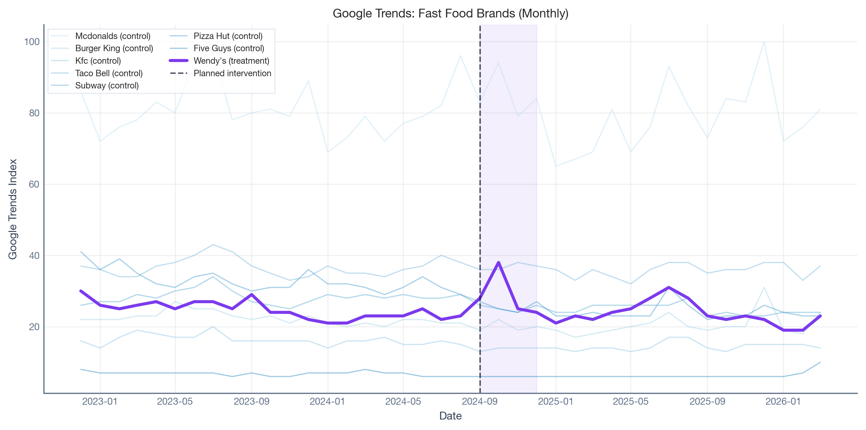
Esto es con lo que estamos trabajando: interés de búsqueda mensual para ocho cadenas de comida rápida desde finales de 2022 hasta principios de 2026. Wendy’s (púrpura) es la marca que ejecutó la campaña; las otras siete son marcas “donantes” potenciales que el Control Sintético combinará para construir un contrafactual.
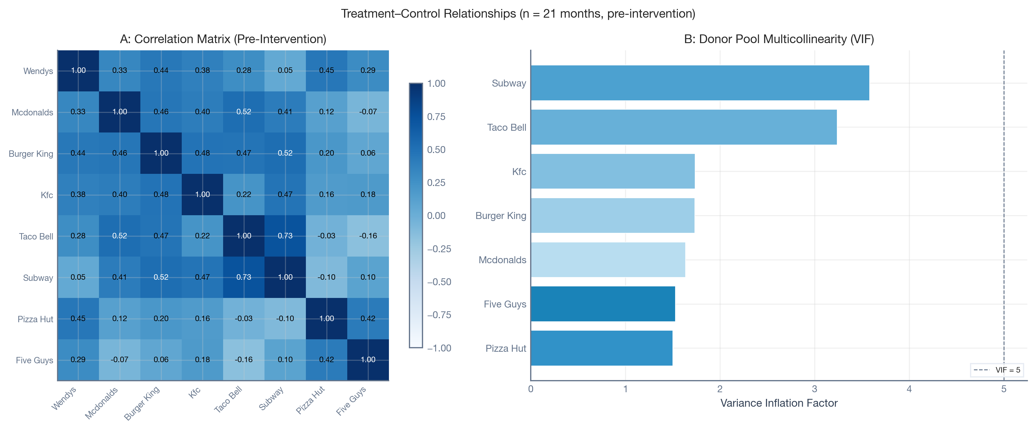
Dos diagnósticos cuentan la historia. La matriz de correlación muestra qué tan fuerte se correlaciona cada marca con Wendy’s — las correlaciones van desde casi cero hasta ~0.45. En términos de pruebas A/B, esto es como tener un grupo control muy ruidoso. Los Factores de Inflación de Varianza muestran cuánto se superponen las marcas control entre sí: un VIF alto significa donantes redundantes.
Show code — correlation matrix and VIF diagnostics
En resumen: Estamos construyendo un contrafactual a partir de predictores mediocres. Eso no es razón para abandonar el análisis — es razón para calibrar cuánto error introduce eso.
El marco
Entradas de diseño
Antes de ejecutar cualquier análisis, deben definirse dos conjuntos de entradas.
Entradas de los interesados (tolerancia al riesgo):
Ancho del ROPE (\Delta): El umbral por debajo del cual un efecto es “prácticamente cero”. Para el caso de Wendy’s, establecemos \Delta = 2.5 puntos de Google Trends, ya que un incremento bimestral menor a 2.5 puntos no es distinguible de manera significativa de la fluctuación orgánica.
Umbral de decisión (p^*): La probabilidad posterior requerida para una decisión definitiva. Usamos p^* = 0.95.
Entradas de conocimiento de dominio (experiencia de mercado):
Prior del efecto esperado (S_{alt}): Una distribución de probabilidad que codifica “si esta campaña funciona, ¿qué tan grande será el incremento?”. Para Wendy’s, el equipo de marketing podría estimar que una campaña viral exitosa debería producir un incremento bimestral en el rango de 5 a 25 puntos de Google Trends.
Calendario placebo (J, L): El número y la longitud de ventanas históricas para calibración. Usamos J = 4 ventanas bimestrales seleccionadas aleatoriamente del período pre-campaña.
Pruebas placebo en el tiempo
La idea central es simple: ejecutar tu estimador en períodos donde sabes que el efecto verdadero es cero. Cualquier estimación distinta de cero revela ruido estructural: la “radiación de fondo” de tu entorno de datos.
Elegimos varias ventanas históricas — períodos bien antes de la campaña real — donde sabemos que el efecto verdadero de tratamiento es cero. Ejecutamos exactamente el mismo modelo de Control Sintético en cada ventana, pretendiendo que una intervención comenzó allí. Lo que el modelo reporta como “efecto causal” se debe enteramente al ruido estructural: tendencias derivando, donantes siendo imperfectos, los supuestos del modelo no cumpliéndose completamente.
Usamos selección aleatoria de pliegues: extraemos tiempos pseudo-intervención uniformemente de meses elegibles (cada uno debe tener al menos el 30% del período pre como datos de entrenamiento, y no puede superponerse con la campaña real). Las ventanas aleatorias muestrean diferentes regímenes estructurales, evitan la correlación temporal entre pliegues adyacentes, y hacen más plausible el supuesto de intercambiabilidad del modelo jerárquico.
La celda de código a continuación define las funciones de utilidad que usaremos a lo largo del resto del análisis — la fábrica de Control Sintético, el ejecutador RandomPlaceboAnalysis, la regla de decisión ROPE, el ajustador nulo jerárquico y el simulador de características operativas.
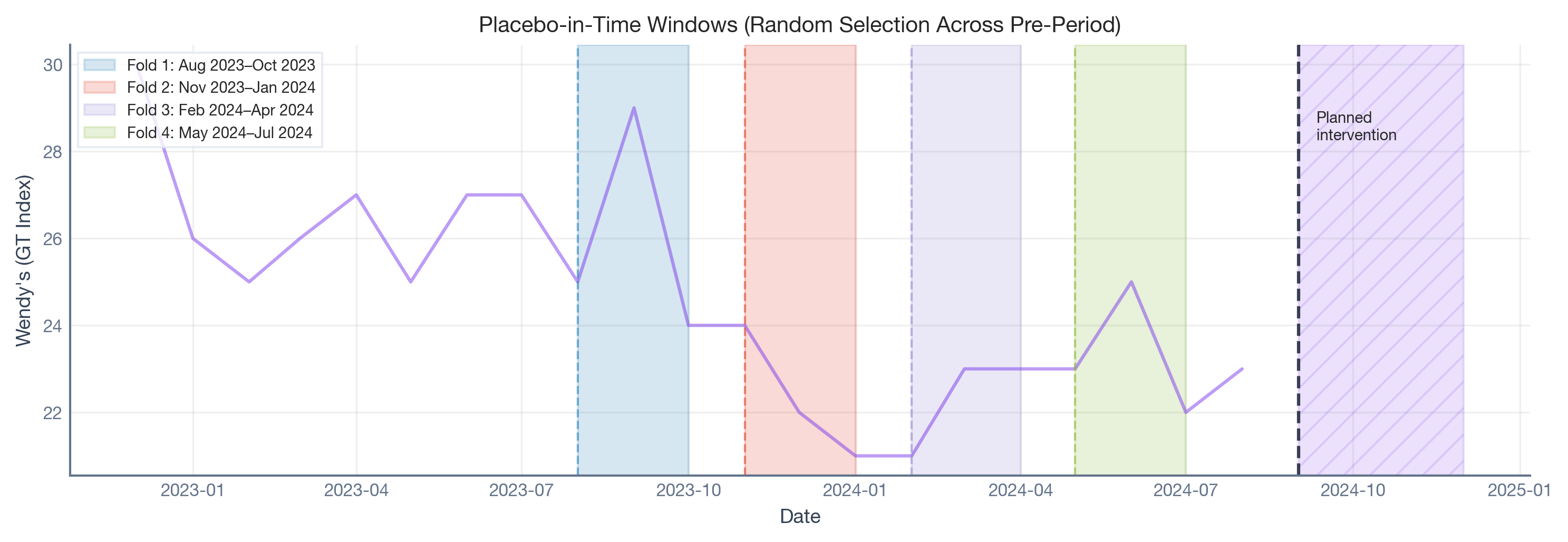
Del período pre-campaña de 21 meses, cuatro tiempos pseudo-intervención fueron seleccionados aleatoriamente (semilla = 42), sujetos a las restricciones de elegibilidad: cada pliegue requiere al menos el 30% de los datos pre-intervención como entrenamiento, y las ventanas placebo no se superponen con el período de intervención. Para cada uno, ajustamos un modelo Bayesiano de Control Sintético (WeightedSumFitter de CausalPy) usando las siete marcas control como unidades donantes.
Show code — run placebo calibration
_pa = RandomPlaceboAnalysis( experiment_factory=sc_factory, dataset=df_pre, intervention_start_date=cfg.INTERVENTION_START, intervention_months=cfg.PLACEBO_MONTHS, n_folds=cfg.N_FOLDS, min_training_pct=cfg.MIN_TRAINING_PCT, min_gap=2, exclude_months=cfg.EXCLUDE_MONTHS, seed=cfg.SEED)results_placebo = _pa.run()print(f"Placebo calibration complete: {len(results_placebo)} folds fitted.")print("Pseudo-intervention start months:",", ".join(r["pseudo_start"].strftime("%b %Y") for r in results_placebo))
El gráfico a continuación muestra qué períodos históricos fueron seleccionados como ventanas placebo. Cada banda de color es una ventana bimestral donde pretendimos que ocurrió una intervención y ejecutamos el pipeline completo de Control Sintético. La región rayada a la derecha es la campaña real de Krabby Patty — completamente intacta durante la calibración.
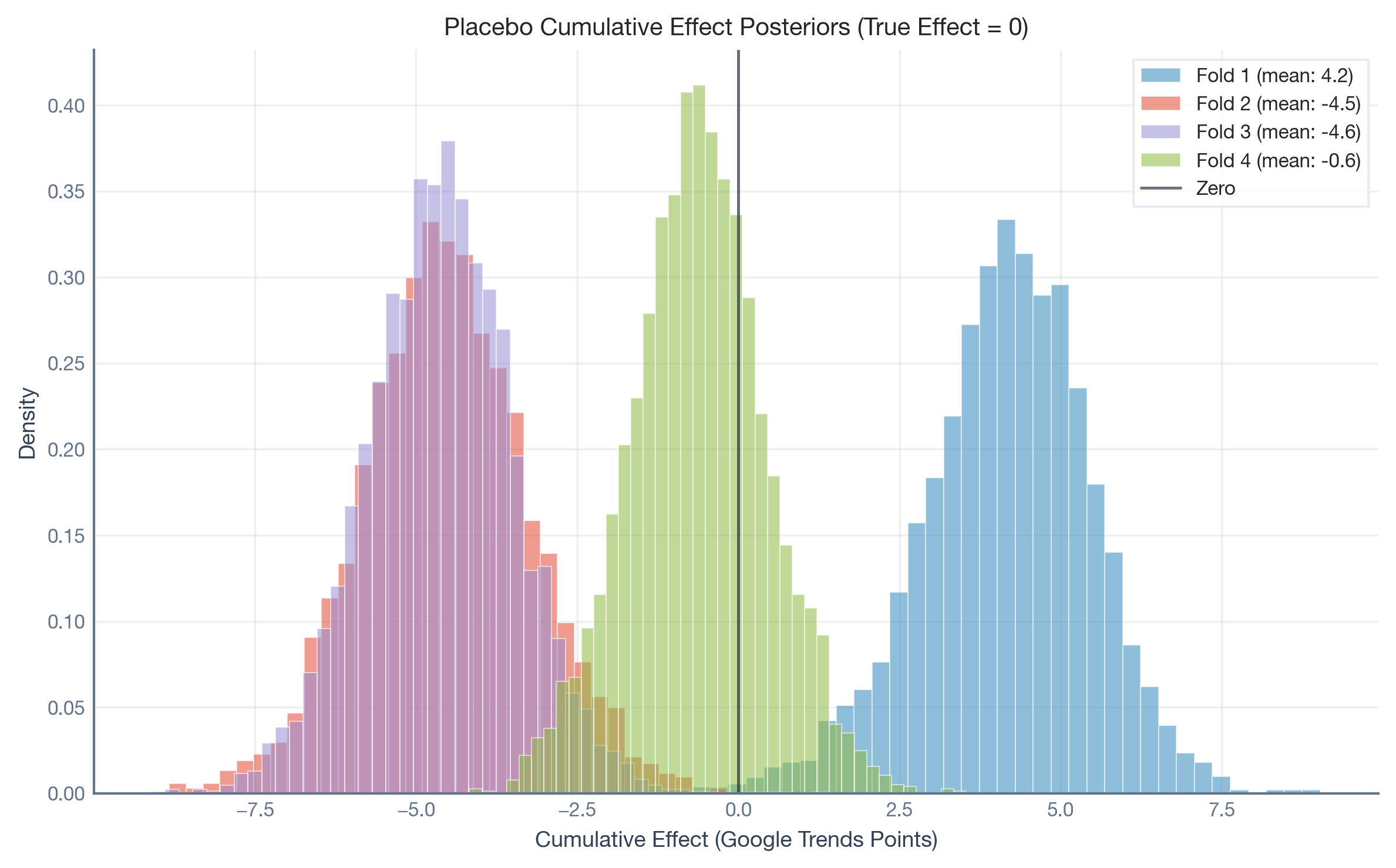
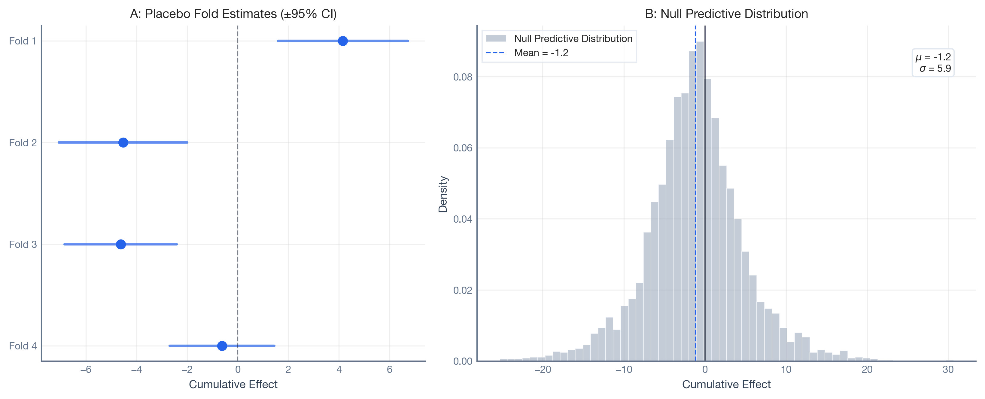
Ahora extraemos los posteriores del efecto acumulado de cada pliegue placebo. Aunque el efecto verdadero es cero en cada ventana, el modelo reporta incrementos estimados que van de aproximadamente -4.7 a +4.2 puntos de Google Trends. El modelo alucina incrementos no triviales a partir de deriva estructural pura.
Show code — extract placebo posteriors
post_impact, fold_means, fold_sds = extract_posteriors(results_placebo)n_samples = post_impact.sizes["sample"]print(f"Fold means: [{', '.join(f'{m:.2f}'for m in fold_means)}]")print(f"Fold SDs: [{', '.join(f'{s:.2f}'for s in fold_sds)}]")
El histograma a continuación muestra la distribución posterior del efecto causal acumulado para cada pliegue placebo. Cada histograma representa un período donde el efecto verdadero es exactamente cero — sin embargo, el modelo reporta efectos no triviales.
Este es el punto clave: los intervalos credibles del modelo son demasiado estrechos para capturar la volatilidad estructural. El posterior de cada pliegue es ajustado (s_j pequeño), pero las medias de los pliegues se dispersan ampliamente. Esta brecha entre la precisión intra-pliegue y la heterogeneidad entre pliegues es exactamente lo que el modelo nulo jerárquico está diseñado para capturar.
Construcción de la nula jerárquica
En lugar de tratar los resultados placebo como anécdotas aisladas (“la peor falsa alarma fue 4.2 puntos”), los modelamos como extracciones de una distribución latente: un proceso de “statu quo” que gobierna cuánta deriva estructural absorbe el estimador.
Esto es similar a un meta-análisis Bayesiano de efectos aleatorios normal–normal (Higgins & Thompson, 2002), donde cada pliegue placebo juega el papel de un “estudio”.
Nivel 1: Incertidumbre intra-pliegue. Para cada pliegue j, la media posterior m_j es una observación ruidosa de un error estructural verdadero latente \theta_j:
\mu_{null}: Sesgo sistemático — la tendencia promedio del modelo a sobre- o subestimar. En un modelo bien calibrado, esto está cerca de cero.
\tau_{het}: Volatilidad estructural — el parámetro crítico. Un \tau_{het} alto significa que el estimador produce rutinariamente falsas alarmas de magnitud no trivial.
Nivel 3: Hiperpriors débilmente informativos. Establecemos \mu_{null} \sim \mathcal{N}(0, 2\hat{\sigma}) y \tau_{het} \sim \text{HalfNormal}(2\hat{\sigma}), donde \hat{\sigma} es la desviación estándar empírica de las medias de los pliegues.
Ajustar este modelo produce una Distribución Predictiva Nula: el rango esperado de estimaciones bajo “sin efecto”:
_draws_per_chain = n_samples // cfg.N_CHAINStheta_new_samples = fit_hierarchical_null(fold_means, fold_sds, _draws_per_chain)_mu_hat =float(np.mean(theta_new_samples))_sd_hat =float(np.std(theta_new_samples))print(f"Null Predictive Distribution fitted.")print(f" mu = {_mu_hat:.2f} GT points (estimator bias)")print(f" sigma = {_sd_hat:.2f} GT points (structural volatility)")print(f" Based on {theta_new_samples.shape[0]:,} posterior draws.")
Sampling: [theta_new]
Null Predictive Distribution fitted.
  mu = -1.16 GT points (estimator bias)
  sigma = 5.90 GT points (structural volatility)
  Based on 4,000 posterior draws.
El gráfico de bosque a continuación (Panel A) muestra el efecto acumulado estimado de cada pliegue placebo con su intervalo credibilidad del 95%. El Panel B muestra la Distribución Predictiva Nula resultante — la mejor estimación del modelo jerárquico de cómo se ve el ruido para este estimador.
Show code — forest plot and null predictive distribution
Esto significa que bajo el statu quo, el estimador puede fácilmente reportar efectos acumulados de +-12 puntos o más, puramente por deriva estructural.
Prior del efecto esperado
El análisis de poder clásico requiere un único tamaño de efecto fijo (“si el incremento real es exactamente 5 puntos, el poder es X%”). En el análisis de diseño Bayesiano, reconocemos que el efecto real de la campaña es incierto incluso si la campaña funciona. Especificamos un Prior del efecto esperadoS_{alt}: una distribución de probabilidad que codifica resultados plausibles bajo la hipótesis alternativa.
Esto nos lleva del Poder clásico a la Assurance Bayesiana (O’Hagan et al., 2005): la probabilidad incondicional de una decisión positiva correcta, promediada sobre todos los tamaños de efecto plausibles. La Assurance responde una pregunta más honesta: “A través del rango realista de resultados de lacampaña, ¿cuál es la probabilidad global de una detección correcta?”
Para el Krabby Patty Kollab, supongamos que el equipo de marketing espera un incremento bimestral en el interés de búsqueda entre 5 y 25 puntos de Google Trends si la campaña es exitosa. Usando un enfoque de Máxima Entropía (PreliZ), encontramos la distribución Gamma menos informativa con el 90% de su masa en [5, 25]:
Show code — expected-effect prior
expected_effect_dist = pz.maxent( pz.Gamma(), lower=cfg.EXPECTED_EFFECT_LOWER, upper=cfg.EXPECTED_EFFECT_UPPER, mass=0.90, plot=False,)_n_draws = theta_new_samples.sizeexpected_effect_samples = expected_effect_dist.rvs( _n_draws, random_state=np.random.default_rng(cfg.SEED),)print(f"Expected-Effect Prior: MaxEnt Gamma with 90% mass in "f"[{cfg.EXPECTED_EFFECT_LOWER}, {cfg.EXPECTED_EFFECT_UPPER}]")print(f" mu = {np.mean(expected_effect_samples):.2f}, "f"sigma = {np.std(expected_effect_samples):.2f}")
Expected-Effect Prior: MaxEnt Gamma with 90% mass in [5.0, 25.0]
  mu = 15.25, sigma = 6.40
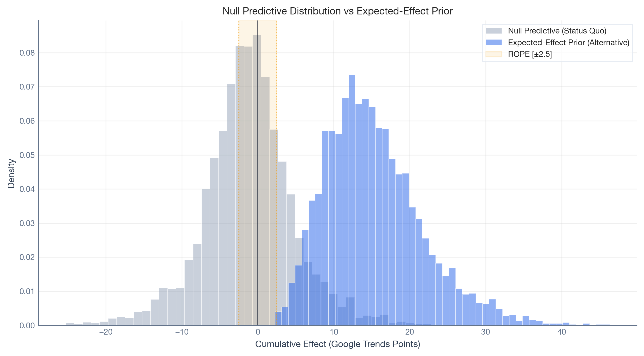
El gráfico a continuación superpone la Distribución Predictiva Nula (gris) con el Prior del Efecto Esperado (azul). La superposición entre ambas distribuciones representa la dificultad fundamental de la tarea de decisión: la zona donde un efecto real de la campaña es difícil de distinguir del ruido estructural.
La práctica estándar en cuasi-experimentos a menudo se basa en una regla binaria: si el intervalo credibilidad del 95% excluye cero, declarar el efecto como significativo. Esto confunde precisión con utilidad: una estimación muy precisa de un incremento de 0.001 puntos es estadísticamente distinta de cero pero prácticamente inútil.
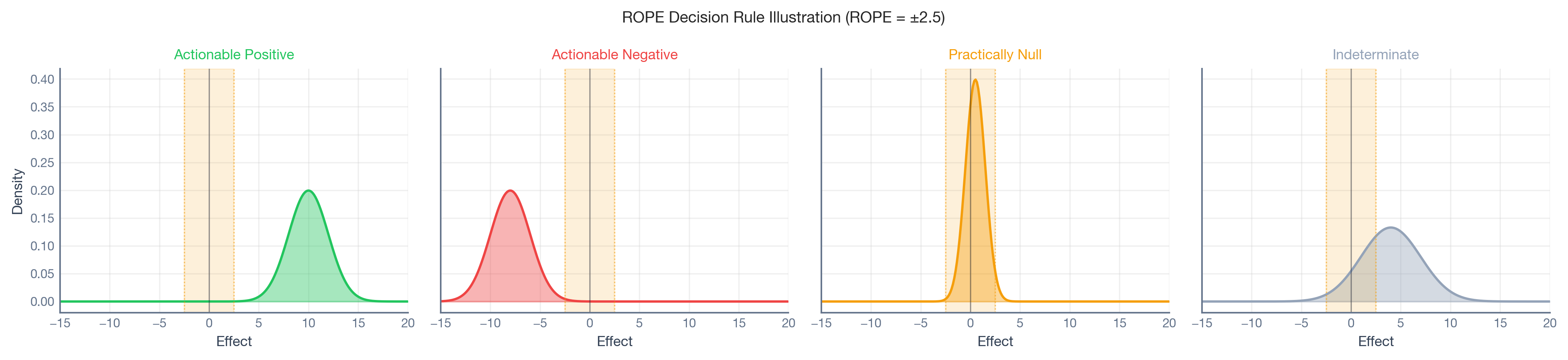
Adoptamos el marco de la Región de Equivalencia Práctica (ROPE) (Kruschke, 2018). Definimos un rango [-\Delta, +\Delta] alrededor de cero que representa efectos que son “prácticamente cero”. La regla de decisión es:
Positivo accionable:P(\hat{\tau} > \Delta) \ge p^* — el efecto supera el umbral práctico con alta confianza.
Nulo práctico:P(|\hat{\tau}| \le \Delta) \ge p^* — el efecto es despreciable.
Indeterminado: De lo contrario — los datos no pueden distinguir señal de ruido.
La clasificación de cuatro categorías introduce explícitamente un resultado de “suspender juicio” y un mecanismo de detección de daño, evitando el modo de falla común donde señales débiles se fuerzan en categorías binarias.
El paso final combina el Nulo Jerárquico, el Prior del Efecto Esperado, y la regla de decisión ROPE en una simulación de Monte Carlo para producir la Tabla de Características Operativas: el perfil de confiabilidad del diseño calculado antes de analizar datos reales de la campaña.
Nota
Algoritmo: simulación Bayesiana de assurance de diseño
Para cada escenario (nula, alternativa), repetir N veces:
Extraer efecto verdadero:\theta^*_i del Predictivo Nulo (nula) o de S_{alt} + Predictivo Nulo (alternativa)
Extraer ruido de estimación:\sigma_i muestreado uniformemente de las desviaciones estándar de los pliegues placebo
Simular posterior sintética: Extraer \hat{\tau}_k \sim \mathcal{N}(\theta^*_i, \sigma_i^2) para k = 1, \dots, K
Clasificar: Aplicar la regla de decisión ROPE
Resultados: Tasa de falsos positivos (nula clasificada como positiva), Assurance Bayesiana (alternativa clasificada como positiva) y tasas de indeterminación para ambos escenarios.
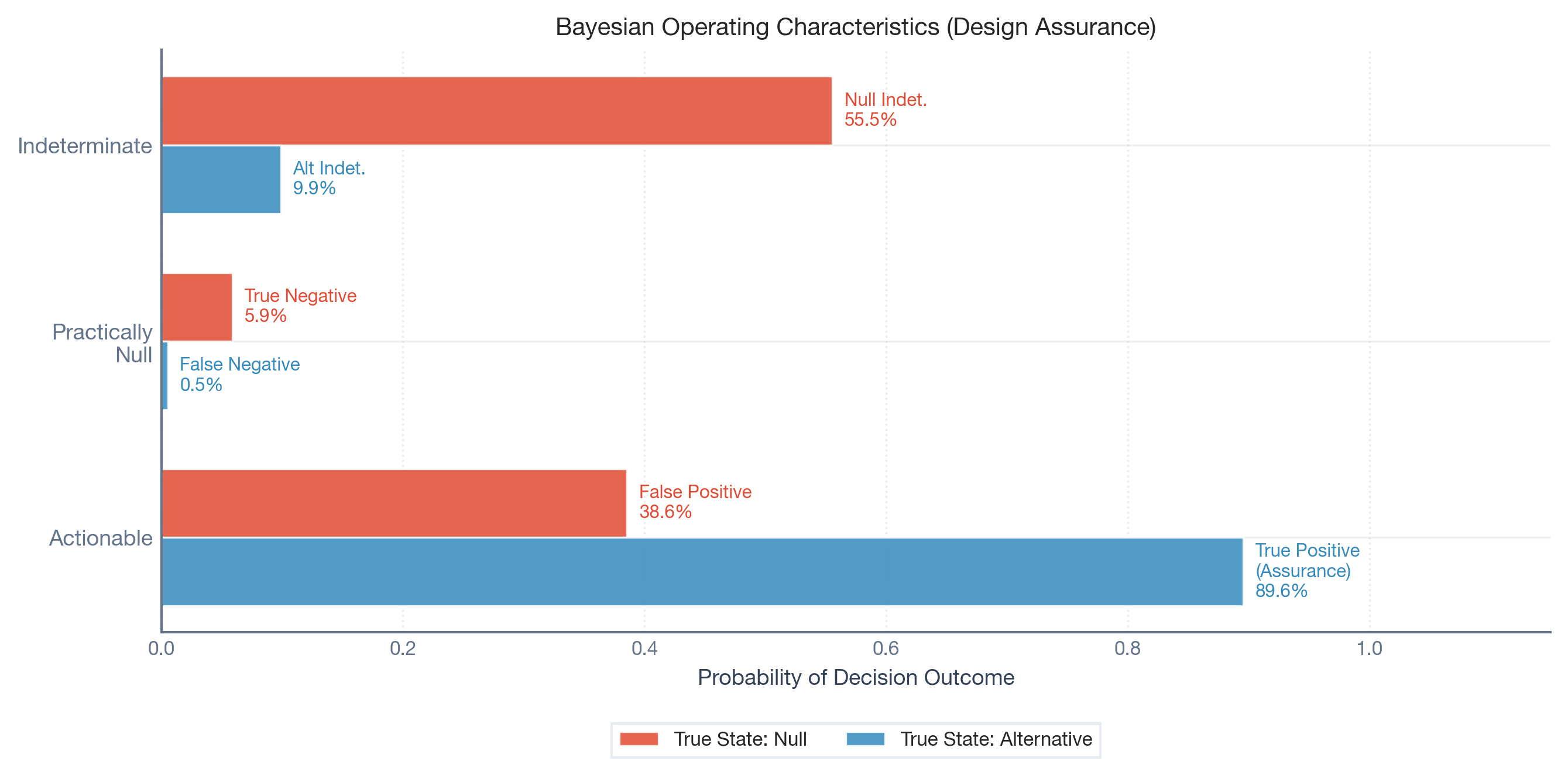
El gráfico a continuación es la salida central del análisis de diseño. Muestra tres resultados de clasificación — Accionable (lo llamaríamos un efecto real), Nulo práctico (diríamos que no pasó nada), e Indeterminado (no podemos decir) — cada uno evaluado bajo dos escenarios: el estado verdadero es nulo (rojo) o alternativa (azul).
Under the status quo, the design erroneously declares an Actionable effect ~41% of the time
Bayesian Assurance
90.1%
If the campaign produces a lift in the expected [5, 25] range, the design detects it with high probability
Null Indeterminacy
53.9%
When there is no effect, 54% of the time the data is simply inconclusive
Alt Indeterminacy
9.3%
When the campaign works, approximately 9% of simulations produce indeterminate results
¿Qué le dice esto al equipo de Wendy’s? El diseño tiene un fuerte poder de detección (90.1% de assurance) pero una tasa de falsos positivos estructurales no trivial (40.8%). Esto es sustancialmente más alto que el umbral convencional del 5% usado en pruebas A/B, y refleja una propiedad genuina de los datos: los índices de Google Trends para cadenas de comida rápida son ruidosos y débilmente correlacionados, haciendo el contrafactual de Control Sintético impreciso.
El resultado: interpretando tu estimación en contexto
Una vez que la campaña se ejecuta y llegan los datos reales, el análisis estándar produce una estimación posterior. Pero ahora el equipo tiene algo que no tenía antes: un sentido calibrado de cuánto confiar en ella.
Todo hasta ahora ha sido calibración pre-intervención. Ahora aplicamos exactamente el mismo estimador de Control Sintético al período real de la campaña (sep–nov 2024) y obtenemos nuestra estimación del efecto de tratamiento.
Un punto crucial: La estimación en sí es idéntica sin importar si realizaste el análisis de diseño. El marco no cambia tu modelo ni ajusta tus números. Proporciona una superposición interpretativa — una etiqueta de confiabilidad que viaja con la estimación.
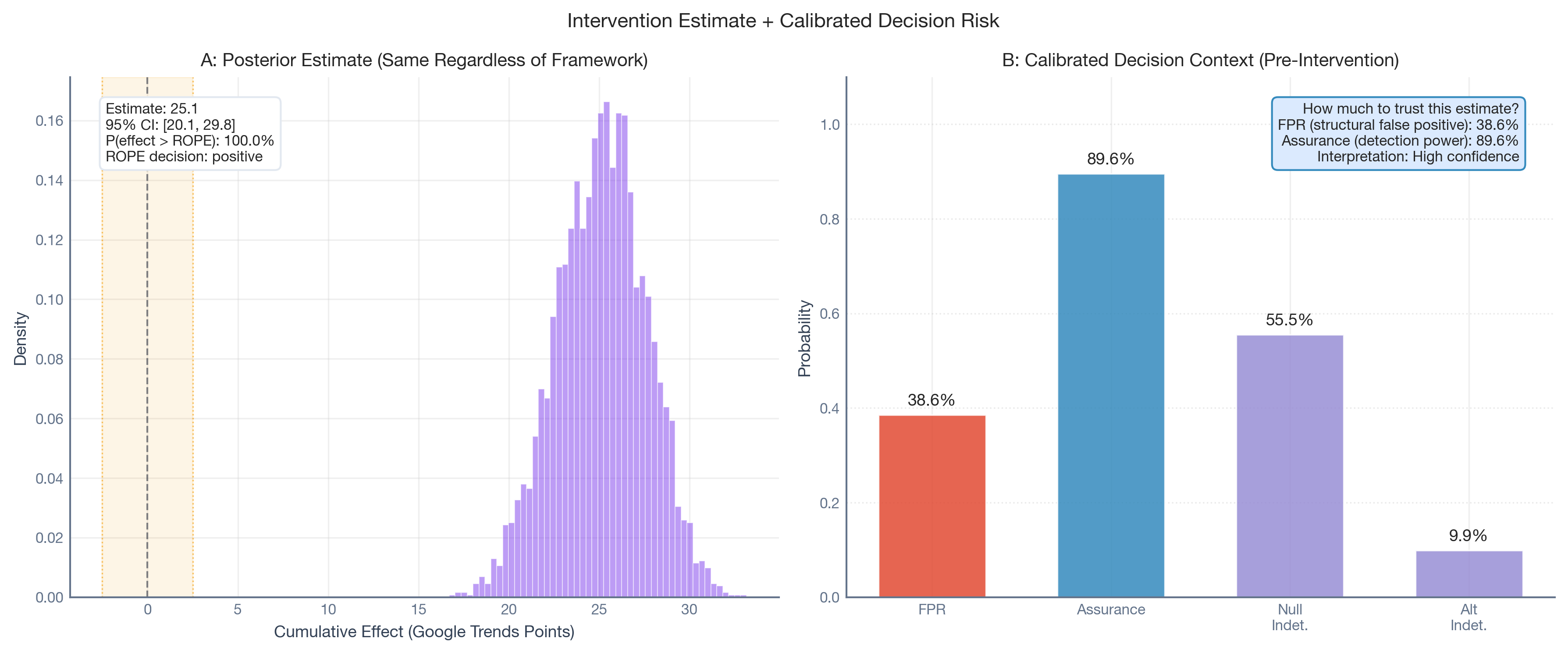
El gráfico a continuación muestra los dos paneles lado a lado. El Panel A es lo que verías sin el marco: una distribución posterior del efecto acumulado. El Panel B es lo que el marco añade: la FPR pre-intervención, la Assurance y las tasas de indeterminación — el contexto que necesitas para interpretar el Panel A con confianza calibrada.
Sin el análisis de diseño, el equipo ve el Panel A: un efecto positivo grande y preciso. Con el análisis de diseño, también ven el Panel B: 90.1% de assurance de que este diseño puede detectar efectos en el rango esperado, atemperado por el conocimiento de que el diseño tiene una FPR estructural del 40.8%. La estimación no cambia, pero la confianza del equipo para interpretarla sí.
La estimación de la intervención de +14.5 puntos GT está muy por encima del ROPE (+-2.5) y dentro del rango del efecto esperado (5–25), lo que convierte esto en un hallazgo de alta confianza incluso dada la FPR elevada. Un efecto observado más pequeño, digamos +4 puntos, justificaría considerablemente más precaución dado el mismo perfil estructural.
Verificaciones de cordura
Antes de actuar basándose en las características operativas, necesitamos responder dos preguntas incómodas:
“¿Solo estoy viendo mi prior?” — Con solo 4 pliegues placebo, el prior del modelo jerárquico para \tau_{het} podría estar determinando los resultados.
“¿Tengo suficientes pliegues placebo?” — Con J = 2 pliegues, la varianza entre pliegues es apenas identificable.
Prueba 1: ¿La escala del prior cambia el resultado?
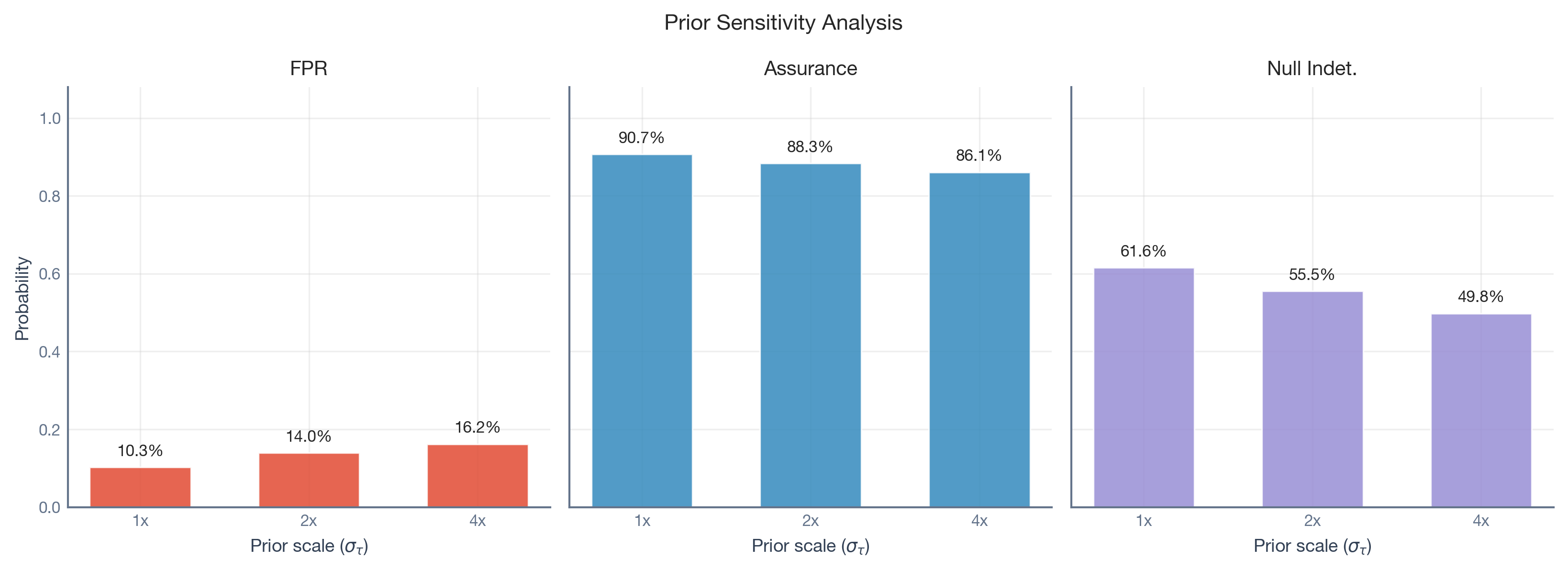
Re-ejecutamos el modelo jerárquico con tres anchos de prior diferentes para \tau_{het}: 1\times, 2\times, y 4\times la desviación estándar empírica de las medias de los pliegues. Si la FPR, la Assurance y la indeterminación son estables a través de un rango de priors de cuatro veces, los datos hablan más fuerte que el prior.
La Assurance es mayormente estable a través de las escalas del prior. La FPR cambia modestamente, confirmando que la tasa elevada de falsos positivos es una propiedad de los datos, no un artefacto del prior.
Prueba 2: ¿Tenemos suficientes pliegues placebo?
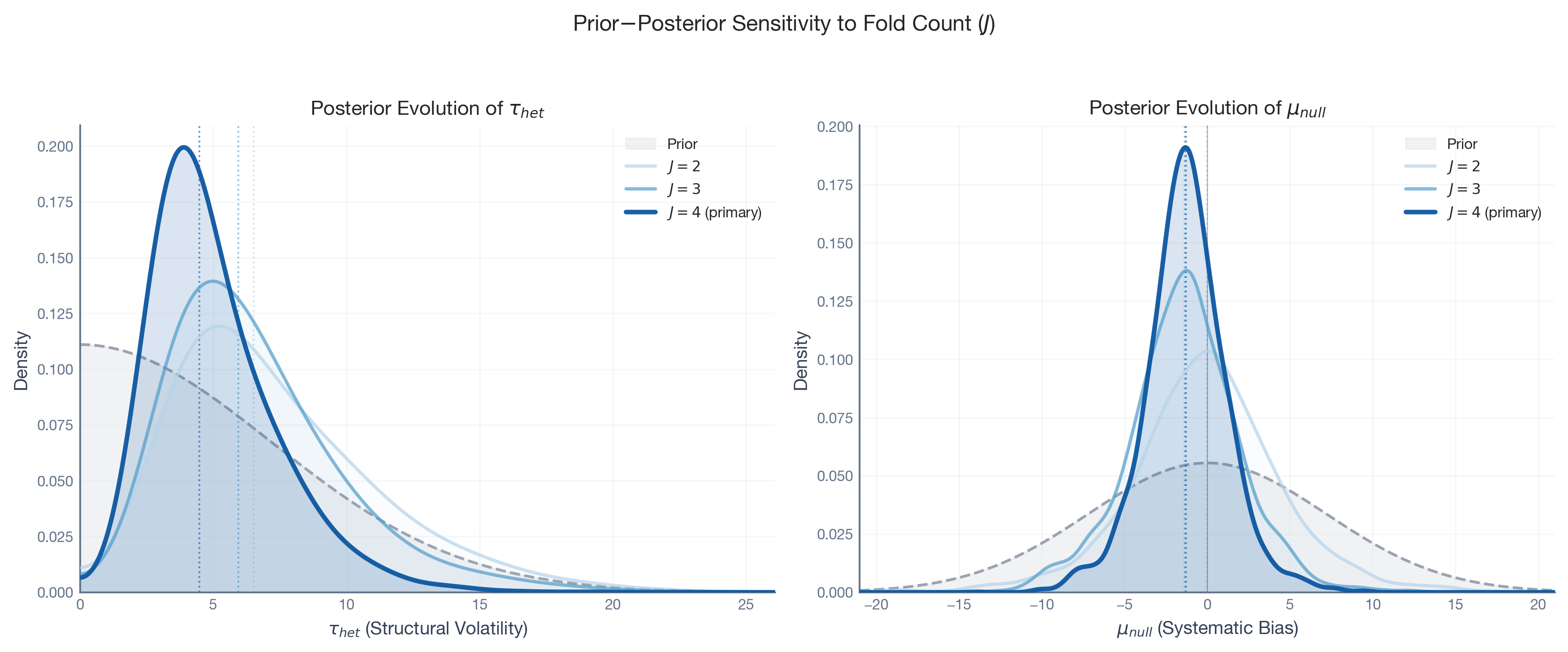
Re-ajustamos el modelo jerárquico usando J = 2, 3, 4 pliegues y observamos cómo \tau_{het} y \mu_{null} evolucionan. Con J = 2, el posterior para \tau_{het} se adhiere a cero — no porque la volatilidad estructural verdadera sea pequeña, sino porque dos puntos de datos no pueden identificar un parámetro de varianza. A medida que añadimos pliegues, el posterior se concentra y estabiliza.
Regla práctica:J \ge 3 es el mínimo para que el marco sea significativo. Con J = 2 estás esencialmente adivinando.
Diagnósticos de especificación: eligiendo el modelo correcto
El marco funciona también como herramienta de selección de modelos. Si las características operativas son insatisfactorias (FPR alta, assurance baja, o indeterminación excesiva), el paso natural siguiente es mejorar el modelo.
El proceso de selección sigue una lógica de “Falsificación y Eficiencia”:
Definir candidatos. Especificar un conjunto de modelos teóricamente distintos. Para Wendy’s, esto podría incluir eliminar marcas débilmente correlacionadas o añadir ajustes estacionales.
Ejecutar calibración placebo para cada uno. Ejecutar el marco completo en cada candidato.
Aplicar criterios de selección: Marcar cualquier modelo donde la FPR supere tu tolerancia. Entre los modelos válidos, preferir el que minimiza \tau_{het} (equivalentemente, maximiza la Assurance).
Para el caso de Wendy’s, las bajas correlaciones sugieren que el contrafactual de Control Sintético está fundamentalmente limitado por el grupo de controles disponible. El diagnóstico de especificación revela esto como una restricción estructural del entorno de datos, no como un error de modelado corregible.
Cerrando el bucle: significancia calibrada post-intervención
Antes de la campaña, preguntamos: “Si hay un efecto real, ¿lo detectaremos?” (Assurance). Ahora la campaña terminó y tenemos una estimación en mano. La pregunta se invierte:
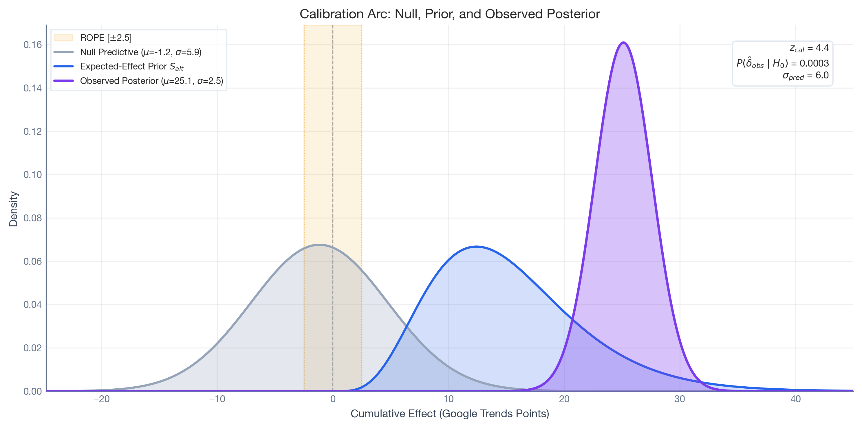
“¿Qué tan probable es que solo el ruido estructural haya producido una estimación tan grande?”
Esta es la probabilidad de cola calibrada — la contraparte post-intervención de la Assurance pre-intervención.
Un p_{cal} pequeño significa que el ruido estructural es extremadamente improbable para explicar el resultado. Uno grande significa que no puedes descartarlo.
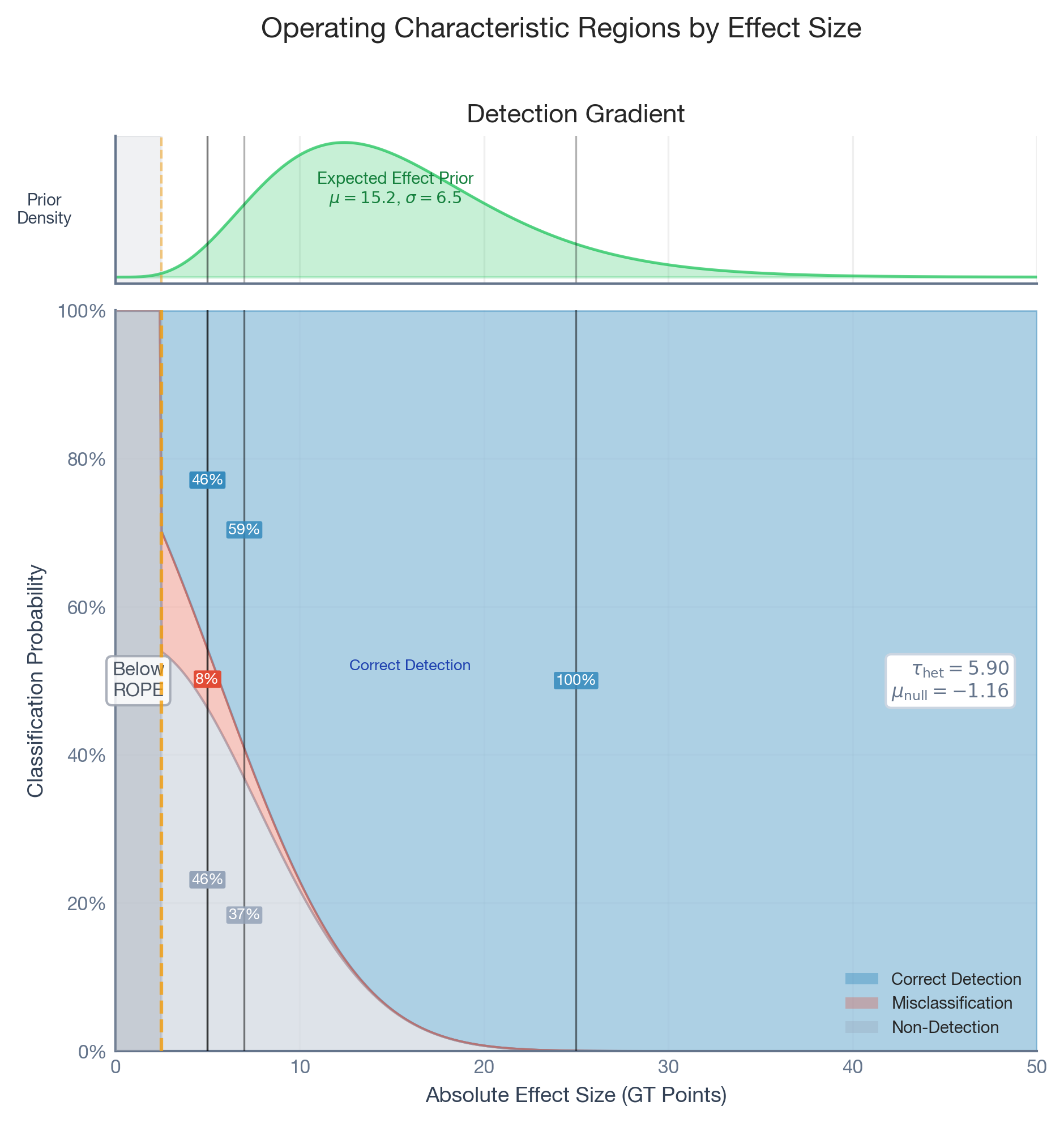
El análisis de poder clásico te da un solo número: el Efecto Mínimo Detectable (MDE). Los efectos por encima de él son “detectables”; por debajo, no lo son. La realidad es más matizada.
El gráfico a continuación muestra la probabilidad de detección como función continua del tamaño del efecto verdadero. En lugar de un umbral binario, obtienes un gradiente: detección correcta (azul), clasificación errónea en la dirección equivocada (rojo), y no detección (gris).
En lugar de preguntar “¿Mi MDE es suficiente?”, puedes preguntar “Con unincremento de 10 puntos, ¿cuál es mi probabilidad de detección? ¿Y con 5 puntos?” Esto es mucho más útil para la toma de decisiones real.
Cuando este marco falla
Cambios de régimen. El marco asume que los errores estructurales durante las ventanas placebo son representativos de aquellos durante el período de intervención. Si la campaña coincide con un quiebre estructural único (un momento viral de la competencia, un shock macroeconómico), la distribución predictiva nula estará miscalibrada.
Demasiado pocos pliegues placebo. Con J < 3, la varianza entre pliegues es esencialmente no identificable. Recomendamos J \ge 3 como mínimo y análisis de sensibilidad sobre la escala del prior para \tau_{het}.
Controles débiles. Cuando las correlaciones tratamiento-control son bajas (como en el caso de Wendy’s), el contrafactual de Control Sintético es impreciso, inflando \tau_{het} y la FPR. El marco diagnostica correctamente esta debilidad pero no puede corregirla; la solución son mejores datos de control, no un mejor procedimiento de calibración.
Entradas erróneas de los interesados. Si el ROPE se establece demasiado estrecho, todo se vuelve indeterminado. Si el prior del efecto esperado se establece demasiado optimista, la assurance se sobreestimará. Estas entradas requieren conocimiento genuino del dominio y deben ser sometidas a pruebas de estrés.
Conclusión
Las estimaciones cuasi-experimentales son tan confiables como el entorno estructural en el que se producen. El marco presentado aquí transforma la pregunta de “¿Es significativo este resultado?” a “¿Qué tan capaz es estediseño específico de distinguir señal de ruido en este entorno de datos específico?”
El caso de estudio de Wendy’s ilustra tanto el poder como las limitaciones del enfoque. El Krabby Patty Kollab produjo una señal (+14.5 puntos GT) lo suficientemente grande como para ser detectada con confianza (90.1% de assurance) a pesar de un entorno de datos con ruido estructural sustancial (40.8% de FPR). Una campaña más débil en el mismo entorno enfrentaría desafíos genuinos de interpretabilidad, y el análisis de diseño lo habría señalado antes del lanzamiento de la campaña.
Animamos a los profesionales a tratar el análisis de diseño como un paso rutinario en cualquier flujo de trabajo cuasi-experimental, no como un ejercicio académico, sino como una auditoría práctica de la confiabilidad de las decisiones.
Disponibilidad de código y datos
Todo el código y datos de este análisis están disponibles en mi repositorio personal. El conjunto de datos de Google Trends es reproducible públicamente. El análisis depende de software de código abierto: PyMC para inferencia Bayesiana, CausalPy para el estimador cuasi-experimental, PreliZ para elicitation de priors, y nutpie para muestreo MCMC.
---title: "Can You Trust Your Quasi-Experiment? A Bayesian Framework for Auditing Time-Series Causal Estimates"date: "2026-04-07"description: "A Bayesian framework using placebo tests and ROPE-based inference to audit whether your quasi-experimental causal estimates are trustworthy."author: - name: Carlos Trujillo - name: Anton Bugaevcategories: [python, experimentation, quasi-experiments, bayesian, pymc]image: "/images/placebo_bayesian_quasi_experiments.jpg"image-alt: "Diagram showing a Bayesian placebo test framework for auditing quasi-experimental causal estimates"jupyter: placebo_bayesian_quasi_experimentsformat: html: code-fold: true code-tools: true code-overflow: wrap---```{python}#| echo: falseimport warningswarnings.filterwarnings("ignore")```## IntroductionIn September 2024, Wendy's launched the "[Krabby Patty Kollab](https://secretatlanta.co/krabby-patties-atlanta/)", a limited-time partnership with Nickelodeon's SpongeBob SquarePants that generated massive buzz across social media and news outlets. Suppose the Wendy's analytics team wanted to measure the campaign's impact on brand search interest using Google Trends data. They can't randomize who sees a viral fast-food collaboration, so they turn to a quasi-experimental design: Synthetic Control, using other fast-food chains as untreated references.The model runs. It reports a cumulative lift of +14.5 Google Trends index points over the campaign month, with a tight 95% credible interval of [12.3, 16.6]. Should they trust this number?The honest answer is: *it depends on the structural reliability of the estimator in this specific data environment.* That tight credible interval captures inherent time-series noise (what statisticians call *aleatoric uncertainty*) and parameter uncertainty (*epistemic uncertainty*), but only conditional on the model's identifying assumptions holding exactly. It says nothing about whether the model itself is trustworthy. When the identifying assumptions are violated — due to seasonal drift, competitor activity, or weak correlations between Wendy's and the control brands — the counterfactual prediction deviates from the true unobserved outcome. We call this deviation the **structural error**, and the broader epistemic uncertainty it reflects **structural uncertainty**. This is what standard quasi-experimental software ignores.This blog presents a framework that quantifies both. By running the same estimator on historical periods where no campaign occurred (placebo tests), pooling those "false alarms" into a hierarchical model, and simulating decision outcomes, we produce a calibrated answer: *"This design has a 40.8% structural false positive rate and 90.1% probability of detecting effects in the expected range."*The framework is:- **Estimator-agnostic.** It wraps around any time-series quasi-experimental method (Interrupted Time Series, Synthetic Control, Difference-in-Differences, Bayesian Structural Time Series) without modifying the estimator itself.- **Pre-intervention.** The entire analysis runs before the campaign launches, enabling go/no-go decisions based on quantified risk.- **Implemented in open-source Python.** PyMC for Bayesian inference, CausalPy for quasi-experimental estimation, PreliZ for prior elicitation, and nutpie for MCMC sampling.::: {.callout-tip}## The Five-Step Recipe1. **Choose your estimator** and define the intervention window length.2. **Run placebo tests** on $J$ historical windows where no treatment occurred.3. **Pool the placebo residuals** into a hierarchical null model to learn the structural volatility.4. **Specify your minimum detectable effect** (ROPE — the band around zero you'd call "practically no effect") and expected lift (alternative hypothesis). We'll formalize this concept in the Decision Rules section below.5. **Simulate operating characteristics.** If assurance is too low or FPR too high, improve the model or reconsider the experiment.Each step is explained below and demonstrated on the Wendy's case study.:::## The Problem: Two Kinds of UncertaintyIf you've designed an A/B test, you've already dealt with **aleatoric uncertainty**: the inherent randomness in your metric. You account for it when you size your test (power analysis) and when you interpret results (confidence or credible intervals). This uncertainty is irreducible: no amount of data collection or modeling can eliminate it.Time-series quasi-experiments have aleatoric uncertainty too. But they have an additional problem: **epistemic uncertainty**, the part of our ignorance that is in principle reducible through better data or better models (Hüllermeier & Waegeman, 2021). Because the counterfactual must be *modeled* rather than *randomized*, the estimate is exposed to a specific form of epistemic uncertainty: the identifying assumptions may be violated. When they are, the counterfactual prediction deviates from the true unobserved outcome. We call this deviation the **structural error**, and the broader uncertainty it reflects **structural uncertainty**. We use *structural* as shorthand throughout this post.Bayesian credible intervals capture aleatoric uncertainty and parameter uncertainty well, but only conditional on the model being correctly specified. If the identifying assumptions break down, the estimator may attribute structural error to the intervention, producing a false positive. The framework presented here empirically characterizes the structural uncertainty distribution by calibrating the estimator against its own historical performance.## Setting Up: Code and DataBefore touching any model, we need to answer a fundamental question: **how good are our control units at predicting the treated unit?** If none of the control brands track Wendy's search interest very well, the synthetic counterfactual will be imprecise — and any gap between real and synthetic could be mistaken for a treatment effect.```{python}#| code-fold: true#| code-summary: "Show code — imports, configuration, and data loading"import contextlibimport iofrom pathlib import Pathfrom typing import Any, Callableimport arviz as azimport causalpy as cpimport matplotlibimport matplotlib.pyplot as pltimport matplotlib.patches as mpatchesimport matplotlib.gridspec as gridspecimport numpy as npimport pandas as pdimport preliz as pzimport pymc as pmimport scipy.stats as statsimport xarray as xrfrom pydantic import BaseModelfrom types import SimpleNamespace# --- Configuration ---_dir = Path("..").resolve()cfg = SimpleNamespace( DATA_PATH="files/google_trends_demo.csv", DPI=300, SEED=42, TREATMENT_COL="wendys", TREATED_UNITS=["wendys"], CONTROL_UNITS=["mcdonalds", "burger_king", "kfc","taco_bell", "subway", "pizza_hut", "five_guys", ], INTERVENTION_START="2024-09-01", INTERVENTION_MONTHS=3, PLACEBO_MONTHS=2, N_FOLDS=4, MIN_TRAINING_PCT=0.30, EXCLUDE_MONTHS={"2024-10", "2024-11"}, ROPE_HALF_WIDTH=2.5, DECISION_THRESHOLD=0.95, EXPECTED_EFFECT_LOWER=5.0, EXPECTED_EFFECT_UPPER=25.0, N_MCMC_DRAWS=1000, N_MCMC_TUNE=1000, N_CHAINS=4, C_TREATMENT="#7c3aed", C_NULL="#94a3b8", C_ALT="#2563eb", C_FPR="#E24A33", C_ASSURANCE="#348ABD", C_INDET="#988ED5", C_NEGATIVE="#b91c1c", C_OTHER_BRANDS="#a8d4f0", BRAND_COLORS={"wendys": "#7c3aed","mcdonalds": "#b8ddf0","burger_king": "#9dcee8","kfc": "#82bfe0","taco_bell": "#67b0d8","subway": "#4ca1d0","pizza_hut": "#3192c8","five_guys": "#1a83b8", }, FOLD_COLORS=["#348ABD", "#E24A33", "#988ED5", "#8EBA42", "#FFB347"],)# --- Plot style ---plt.style.use("seaborn-v0_8-whitegrid")plt.rcParams.update({"figure.figsize": [9, 5],"figure.dpi": 150,"font.family": "sans-serif","font.sans-serif": ["Source Sans Pro", "Helvetica Neue", "Arial"],"font.size": 9,"axes.labelsize": 9,"axes.titlesize": 10,"axes.titleweight": "bold","xtick.labelsize": 8,"ytick.labelsize": 8,"legend.fontsize": 8,"figure.titlesize": 11,"axes.spines.top": False,"axes.spines.right": False,"axes.edgecolor": "#64748b","axes.labelcolor": "#334155","xtick.color": "#64748b","ytick.color": "#64748b","grid.alpha": 0.3,})# --- Load data ---df = pd.read_csv(cfg.DATA_PATH, parse_dates=["Time"])df.columns = ["date", "mcdonalds", "burger_king", "wendys", "kfc","taco_bell", "subway", "pizza_hut", "five_guys",]df = df.set_index("date").sort_index().astype(float)intervention_ts = pd.Timestamp(cfg.INTERVENTION_START)df_pre = df.loc[df.index < intervention_ts].copy()print(f"Data loaded: {len(df)} months ({df.index.min():%Y-%m} to {df.index.max():%Y-%m}).")print(f"Pre-intervention: {len(df_pre)} months available for calibration.")```### The raw data: eight fast-food brands on Google TrendsHere's what we're working with: monthly search interest for eight fast-food brands from late 2022 through early 2026. Wendy's (purple) is the brand that ran the campaign; the other seven are potential "donor" brands that the Synthetic Control will blend together to build a counterfactual.```{python}#| code-fold: true#| code-summary: "Show code — raw data plot"fig, ax = plt.subplots(figsize=(10, 5))for brand in cfg.CONTROL_UNITS: ax.plot( df.index, df[brand], color=cfg.BRAND_COLORS.get(brand, cfg.C_OTHER_BRANDS), alpha=0.4, linewidth=1, label=brand.replace("_", " ").title() +" (control)", )ax.plot( df.index, df[cfg.TREATMENT_COL], color=cfg.C_TREATMENT, linewidth=2.5, label="Wendy's (treatment)",)ax.axvline( intervention_ts, color="#0f172a", linestyle="--", linewidth=1.2, alpha=0.7, label="Planned intervention",)ax.axvspan( intervention_ts, intervention_ts + pd.DateOffset(months=cfg.INTERVENTION_MONTHS), alpha=0.08, color=cfg.C_TREATMENT,)ax.set_xlabel("Date")ax.set_ylabel("Google Trends Index")ax.set_title("Google Trends: Fast Food Brands (Monthly)")ax.legend( loc="upper left", frameon=True, fancybox=False, edgecolor="#e2e8f0", fontsize=7, ncol=2,)fig.tight_layout()plt.show()```### How well do the controls predict Wendy's?Two diagnostics tell the story. The **correlation matrix** shows how strongly each brand correlates with Wendy's — correlations range from near-zero to ~0.45. In A/B testing terms, this is like having a very noisy control group. The **Variance Inflation Factors** show how much the control brands overlap with each other: high VIF means redundant donors.```{python}#| code-fold: true#| code-summary: "Show code — correlation matrix and VIF diagnostics"_cols = [cfg.TREATMENT_COL] + cfg.CONTROL_UNITS_corr = df_pre[_cols].corr()fig, (ax_heat, ax_vif) = plt.subplots(1, 2, figsize=(12, 5), gridspec_kw={"width_ratios": [1, 1.2]},)# Panel A: Correlation heatmapim = ax_heat.imshow( _corr.values, cmap="Blues", vmin=-1, vmax=1, aspect="auto",)_labels = [c.replace("_", " ").title() for c in _cols]ax_heat.set_xticks(range(len(_cols)))ax_heat.set_yticks(range(len(_cols)))ax_heat.set_xticklabels(_labels, rotation=45, ha="right", fontsize=7)ax_heat.set_yticklabels(_labels, fontsize=7)for i inrange(len(_cols)):for j inrange(len(_cols)): ax_heat.text( j, i, f"{_corr.values[i, j]:.2f}", ha="center", va="center", fontsize=6.5, color="white"ifabs(_corr.values[i, j]) >0.5else"black", )fig.colorbar(im, ax=ax_heat, shrink=0.8)ax_heat.set_title("A: Correlation Matrix (Pre-Intervention)")# Panel B: VIF_X_ctrl = df_pre[cfg.CONTROL_UNITS].valuesvifs = {}for j_idx, ctrl inenumerate(cfg.CONTROL_UNITS): _y_j = _X_ctrl[:, j_idx] _X_rest = np.delete(_X_ctrl, j_idx, axis=1) _X_rest = np.column_stack([np.ones(_X_rest.shape[0]), _X_rest]) _coef, *_ = np.linalg.lstsq(_X_rest, _y_j, rcond=None) _ss_res = np.sum((_y_j - _X_rest @ _coef) **2) _ss_tot = np.sum((_y_j - _y_j.mean()) **2) _r_sq =1- _ss_res / _ss_tot if _ss_tot >0else0.0 vifs[ctrl] =1.0/ (1.0- _r_sq) if _r_sq <1.0else np.inf_sorted_brands =sorted(vifs, key=vifs.get)_vif_vals = [vifs[b] for b in _sorted_brands]_bar_colors = [cfg.BRAND_COLORS.get(b, cfg.C_OTHER_BRANDS) for b in _sorted_brands]_bar_labels = [b.replace("_", " ").title() for b in _sorted_brands]ax_vif.barh( _bar_labels, _vif_vals, color=_bar_colors, edgecolor="white", linewidth=0.5,)ax_vif.axvline(5, color="#64748b", linestyle="--", linewidth=0.8, label="VIF = 5",)ax_vif.set_xlabel("Variance Inflation Factor")ax_vif.set_title("B: Donor Pool Multicollinearity (VIF)")ax_vif.legend( frameon=True, fancybox=False, edgecolor="#e2e8f0", fontsize=6.5, loc="lower right",)fig.suptitle(f"Treatment\u2013Control Relationships "f"(n = {len(df_pre)} months, pre-intervention)", fontweight="bold", fontsize=10,)fig.tight_layout()plt.show()```**Bottom line:** We're building a counterfactual from mediocre predictors. That's not a reason to abandon the analysis — it's a reason to *calibrate how much error that introduces*.## The Framework### Design InputsBefore running any analysis, two sets of inputs must be defined.**Stakeholder inputs** (risk tolerance):- **ROPE half-width ($\Delta$):** The threshold below which an effect is "practically zero." For the Wendy's case, we set $\Delta = 2.5$ Google Trends points, as a bimonthly lift smaller than 2.5 points is not meaningfully distinguishable from organic fluctuation.- **Decision threshold ($p^*$):** The required posterior probability for a definitive call. We use $p^* = 0.95$.**Domain-knowledge inputs** (market expertise):- **Expected-Effect Prior ($S_{alt}$):** A probability distribution encoding "if this campaign works, how big will the lift be?" For Wendy's, the marketing team might judge that a successful viral campaign should produce a bimonthly lift in the range of 5 to 25 GT points.- **Placebo schedule ($J$, $L$):** The number and length of historical windows for calibration. We use $J = 4$ bimonthly windows randomly selected from the pre-campaign period.### Placebo-in-Time TestsThe core idea is simple: run your estimator on periods where you *know* the true effect is zero. Any non-zero estimate reveals structural noise: the "background radiation" of your data environment.We pick several historical windows — periods well before the actual campaign — where we *know* the true treatment effect is zero. We run the exact same Synthetic Control model on each window, pretending an intervention started there. Whatever the model reports as a "causal effect" is entirely due to structural noise: trends drifting, donors being imperfect, the model's assumptions not quite holding.We use **random** fold selection: we draw pseudo-intervention times uniformly from eligible months (each must have at least 30% of the pre-period as training data, and can't overlap the real campaign). Random windows sample different structural regimes, avoid temporal correlation between adjacent folds, and make the exchangeability assumption of the hierarchical model more plausible.The code cell below defines the utility functions we'll use throughout the rest of the analysis — the Synthetic Control factory, the RandomPlaceboAnalysis runner, the ROPE decision rule, the hierarchical null fitter, and the operating characteristics simulator.```{python}#| output: false#| code-fold: true#| code-summary: "Show code — utility functions"# --- Synthetic Control factory ---def sc_factory(dataset, treatment_time, treatment_time_end):"""CausalPy Synthetic Control factory."""return cp.SyntheticControl( dataset, treatment_time, control_units=cfg.CONTROL_UNITS, treated_units=cfg.TREATED_UNITS, model=cp.pymc_models.WeightedSumFitter( sample_kwargs={"target_accept": 0.95,"random_seed": cfg.SEED,"progressbar": False, } ), )# --- Random Placebo Analysis ---class RandomPlaceboAnalysis(BaseModel):"""Placebo-in-time analysis with randomly selected windows.""" model_config = {"arbitrary_types_allowed": True} experiment_factory: Callable dataset: pd.DataFrame intervention_start_date: str intervention_months: int=1 n_folds: int=4 min_training_pct: float=0.30 min_gap: int=1 exclude_months: set[str] |None=None seed: int=42def run(self) ->list[dict[str, Any]]: treatment_time = pd.Timestamp(self.intervention_start_date) pre_df =self.dataset.loc[self.dataset.index < treatment_time].copy()if pre_df.empty:raiseValueError("No observations before treatment_time.") n_total =len(pre_df) min_training =int(np.ceil(self.min_training_pct * n_total)) exclude =self.exclude_months orset() all_dates = pre_df.index.sort_values() candidates = []for date in all_dates: pseudo_end = date + pd.DateOffset(months=self.intervention_months)if date.strftime("%Y-%m") in exclude:continue n_pre = (all_dates < date).sum()if n_pre < min_training:continueif pseudo_end > treatment_time:continue candidates.append(date)iflen(candidates) <self.n_folds:raiseValueError(f"Only {len(candidates)} eligible periods, "f"but {self.n_folds} folds requested." ) rng = np.random.default_rng(self.seed) pool =list(range(len(candidates))) selected_idx = []for _ inrange(self.n_folds): valid = [ i for i in poolifall(abs(i - s) >=self.min_gap for s in selected_idx) ]ifnot valid:raiseValueError("Cannot select enough folds with min_gap constraint." ) pick = rng.choice(valid) selected_idx.append(pick) pool.remove(pick) selected =sorted([candidates[i] for i in selected_idx]) results = []for fold_idx, pseudo_start inenumerate(selected, 1): pseudo_end = pseudo_start + pd.DateOffset(months=self.intervention_months) fold_df = pre_df.loc[pre_df.index < pseudo_end].sort_index() result =self.experiment_factory(fold_df, pseudo_start, pseudo_end) results.append({"fold": fold_idx,"pseudo_start": pseudo_start,"pseudo_end": pseudo_end,"result": result, })return results# --- ROPE decision rule ---def bayesian_rope_decision(samples, rope_half_width, threshold):"""Classify a posterior sample under the ROPE decision rule."""if samples.ndim !=1: samples = np.asarray(samples).ravel() prob_pos = (samples > rope_half_width).mean() prob_neg = (samples <-rope_half_width).mean() prob_null = (np.abs(samples) <= rope_half_width).mean()if prob_pos >= threshold:return"positive"elif prob_neg >= threshold:return"negative"elif prob_null >= threshold:return"null"else:return"indeterminate"# --- Extract posteriors from placebo results ---def extract_posteriors(results):"""Extract cumulative posterior summaries from placebo fold results.""" post_impact = xr.concat( [ r["result"] .post_impact.sum("obs_ind") .isel(treated_units=0) .stack(sample=("chain", "draw"))for r in results ], dim="fold", ) post_impact = post_impact.assign_coords( sample=np.arange(post_impact.sizes["sample"]) ) n_folds = post_impact.sizes["fold"] fold_means = np.array([ post_impact.isel(fold=i).mean().item() for i inrange(n_folds) ]) fold_sds = np.array([ post_impact.isel(fold=i).std().item() for i inrange(n_folds) ]) fold_sds = np.where(fold_sds <1e-6, 1e-6, fold_sds)return post_impact, fold_means, fold_sds# --- Hierarchical null model ---def fit_hierarchical_null(fold_means, fold_sds, draws_per_chain):"""Fit hierarchical normal-normal null model; return theta_new samples.""" n_folds =len(fold_means) prior_mu_scale = (float(np.nanstd(fold_means)) if np.nanstd(fold_means) >0else1.0 ) coords = {"fold": np.arange(n_folds)}with pm.Model(coords=coords) as model: pm.Data("obs_means", fold_means, dims="fold") obs_sd = pm.Data("obs_sd", fold_sds, dims="fold") mu = pm.Normal("mu", mu=0.0, sigma=2.0* prior_mu_scale) tau = pm.HalfNormal("tau", sigma=2.0* prior_mu_scale) z = pm.Normal("z", mu=0.0, sigma=1.0, dims="fold") theta = pm.Deterministic("theta", mu + tau * z, dims="fold") pm.Normal("lik", mu=theta, sigma=obs_sd, observed=fold_means, dims="fold", ) idata = pm.sample( draws=draws_per_chain, tune=cfg.N_MCMC_TUNE, chains=cfg.N_CHAINS, target_accept=0.97, nuts_sampler="nutpie", random_seed=cfg.SEED, progressbar=False )with model: model.add_coords({"new": np.arange(1)}) pm.Normal("theta_new", mu=mu, sigma=tau, dims="new") ppc = pm.sample_posterior_predictive( idata, var_names=["theta_new"], random_seed=cfg.SEED, progressbar=False, )return ( ppc["posterior_predictive"]["theta_new"] .stack(sample=("chain", "draw")).values.squeeze() )# --- Operating characteristics simulator ---def compute_oc(theta_new_samples, fold_sds, expected_effect_samples, n_samples_total):"""Compute operating characteristics via ROPE simulation.""" n_reps =int(min(theta_new_samples.size, expected_effect_samples.size)) rng = np.random.default_rng(cfg.SEED) null_decisions, alt_decisions = [], []for i inrange(n_reps): sd_sim = rng.choice(fold_sds) post_null = rng.normal(float(theta_new_samples[i]), sd_sim, size=n_samples_total, ) null_decisions.append( bayesian_rope_decision(post_null, cfg.ROPE_HALF_WIDTH, cfg.DECISION_THRESHOLD) ) post_alt = rng.normal(float(expected_effect_samples[i] + theta_new_samples[i]), sd_sim, size=n_samples_total, ) alt_decisions.append( bayesian_rope_decision(post_alt, cfg.ROPE_HALF_WIDTH, cfg.DECISION_THRESHOLD) ) null_decisions = np.array(null_decisions) alt_decisions = np.array(alt_decisions) _null_act = (null_decisions =="positive") | (null_decisions =="negative") _alt_act = (alt_decisions =="positive") | (alt_decisions =="negative")return {"FPR": float(np.mean(_null_act)),"Assurance": float(np.mean(_alt_act)),"Null Indet.": float(np.mean(null_decisions =="indeterminate")),"Alt Indet.": float(np.mean(alt_decisions =="indeterminate")),"Null True Neg.": float(np.mean(null_decisions =="null")),"Alt False Neg.": float(np.mean(alt_decisions =="null")),"null_decisions": null_decisions,"alt_decisions": alt_decisions, }```#### Running the Placebo TestsFrom the 21-month pre-campaign period, four pseudo-intervention times were randomly selected (seed = 42), subject to the eligibility constraints: each fold requires at least 30% of pre-intervention data as training, and the placebo windows do not overlap with the intervention period. For each, we fit a Bayesian Synthetic Control model (CausalPy's `WeightedSumFitter`) using the seven control brands as donor units.```{python}#| output: false#| code-fold: true#| code-summary: "Show code — run placebo calibration"_pa = RandomPlaceboAnalysis( experiment_factory=sc_factory, dataset=df_pre, intervention_start_date=cfg.INTERVENTION_START, intervention_months=cfg.PLACEBO_MONTHS, n_folds=cfg.N_FOLDS, min_training_pct=cfg.MIN_TRAINING_PCT, min_gap=2, exclude_months=cfg.EXCLUDE_MONTHS, seed=cfg.SEED)results_placebo = _pa.run()print(f"Placebo calibration complete: {len(results_placebo)} folds fitted.")print("Pseudo-intervention start months:",", ".join(r["pseudo_start"].strftime("%b %Y") for r in results_placebo))```The plot below shows which historical periods were selected as placebo windows. Each colored band is a bimonthly window where we *pretended* an intervention happened and ran the full Synthetic Control pipeline. The hatched region on the right is the actual Krabby Patty campaign — completely untouched during calibration.```{python}#| code-fold: true#| code-summary: "Show code — placebo windows schematic"fig, ax = plt.subplots(figsize=(10, 3.5))_dates = df_pre.indexax.plot( _dates, df_pre[cfg.TREATMENT_COL], color=cfg.C_TREATMENT, linewidth=1.5, alpha=0.5,)for i, r inenumerate(results_placebo): ps = r["pseudo_start"] pe = r["pseudo_end"] c = cfg.FOLD_COLORS[i %len(cfg.FOLD_COLORS)] ax.axvspan( ps, pe, alpha=0.2, color=c, label=f"Fold {i+1}: {ps.strftime('%b %Y')}\u2013{pe.strftime('%b %Y')}", ) ax.axvline(ps, color=c, linewidth=1, linestyle="--", alpha=0.6)ax.axvspan( intervention_ts, intervention_ts + pd.DateOffset(months=cfg.INTERVENTION_MONTHS), alpha=0.15, color=cfg.C_TREATMENT, hatch="//",)ax.axvline( intervention_ts, color="#0f172a", linewidth=1.5, linestyle="--", alpha=0.8,)ax.text( intervention_ts + pd.DateOffset(days=10), ax.get_ylim()[1] *0.95,"Planned\nintervention", fontsize=7, va="top", fontweight="bold",)ax.set_xlabel("Date")ax.set_ylabel("Wendy's (GT Index)")ax.set_title("Placebo-in-Time Windows (Random Selection Across Pre-Period)")ax.legend( loc="upper left", fontsize=7, frameon=True, fancybox=False, edgecolor="#e2e8f0",)fig.tight_layout()plt.show()```Now we extract the cumulative effect posteriors from each placebo fold. Even though the true effect is zero in every window, the model reports estimated lifts ranging from approximately −4.7 to +4.2 Google Trends points. The model hallucinates non-trivial lifts from pure structural drift.```{python}#| code-fold: true#| code-summary: "Show code — extract placebo posteriors"post_impact, fold_means, fold_sds = extract_posteriors(results_placebo)n_samples = post_impact.sizes["sample"]print(f"Fold means: [{', '.join(f'{m:.2f}'for m in fold_means)}]")print(f"Fold SDs: [{', '.join(f'{s:.2f}'for s in fold_sds)}]")```The histogram below shows the posterior distribution of the cumulative causal effect for each placebo fold. Each histogram represents a period where **the true effect is exactly zero** — yet the model reports non-trivial effects.```{python}#| code-fold: true#| code-summary: "Show code — placebo posteriors histogram"_n_folds = post_impact.sizes["fold"]fig, ax = plt.subplots(figsize=(8, 5))for i inrange(_n_folds): _data = post_impact.isel(fold=i).values ax.hist( _data, bins=40, density=True, alpha=0.55, color=cfg.FOLD_COLORS[i %len(cfg.FOLD_COLORS)], edgecolor="white", linewidth=0.5, label=f"Fold {i+1} (mean: {fold_means[i]:.1f})", )ax.axvline(0, color="#0f172a", linestyle="-", linewidth=1.2, alpha=0.6, label="Zero")ax.set_xlabel("Cumulative Effect (Google Trends Points)")ax.set_ylabel("Density")ax.set_title("Placebo Cumulative Effect Posteriors (True Effect = 0)")ax.legend(frameon=True, fancybox=False, edgecolor="#e2e8f0")fig.tight_layout()plt.show()```**This is the key insight:** the model's credible intervals are too narrow to capture the structural volatility. Each fold's posterior is tight (small $s_j$), but the fold means scatter widely. This gap between within-fold precision and between-fold heterogeneity is exactly what the hierarchical null model is designed to capture.### Hierarchical Null ConstructionRather than treating placebo results as isolated anecdotes ("the worst false alarm was 4.2 points"), we model them as draws from a latent distribution: a "status quo" process governing how much structural drift the estimator absorbs.This is similar to a Bayesian normal–normal random-effects meta-analysis (Higgins & Thompson, 2002), where each placebo fold plays the role of a "study."**Level 1: Within-fold uncertainty.** For each fold $j$, the posterior mean $m_j$ is a noisy observation of a latent true structural error $\theta_j$:$$m_j \mid \theta_j, s_j \sim \mathcal{N}(\theta_j,\; s_j^2)$$**Level 2: Between-fold heterogeneity.** The latent errors are drawn from a population distribution:$$\theta_j \sim \mathcal{N}(\mu_{null},\; \tau_{het}^2)$$- $\mu_{null}$: Systematic bias — the model's average tendency to over- or under-estimate. In a well-calibrated model, this is near zero.- $\tau_{het}$: Structural volatility — the critical parameter. A high $\tau_{het}$ means the estimator routinely produces false alarms of non-trivial magnitude.**Level 3: Weakly informative hyperpriors.** We set $\mu_{null} \sim \mathcal{N}(0, 2\hat{\sigma})$ and $\tau_{het} \sim \text{HalfNormal}(2\hat{\sigma})$, where $\hat{\sigma}$ is the empirical standard deviation of the fold means.Fitting this model yields a **Null Predictive Distribution**: the expected range of estimates under "no effect":$$\tilde{\theta}_{new} \sim \mathcal{N}(\mu_{null},\; \tau_{het}^2)$$```{python}#| code-fold: true#| code-summary: "Show code — fit hierarchical null model"_draws_per_chain = n_samples // cfg.N_CHAINStheta_new_samples = fit_hierarchical_null(fold_means, fold_sds, _draws_per_chain)_mu_hat =float(np.mean(theta_new_samples))_sd_hat =float(np.std(theta_new_samples))print(f"Null Predictive Distribution fitted.")print(f" mu = {_mu_hat:.2f} GT points (estimator bias)")print(f" sigma = {_sd_hat:.2f} GT points (structural volatility)")print(f" Based on {theta_new_samples.shape[0]:,} posterior draws.")```The forest plot below (Panel A) shows each placebo fold's estimated cumulative effect with its 95% credible interval. Panel B shows the resulting Null Predictive Distribution — the hierarchical model's best estimate of *what noise looks like* for this estimator.```{python}#| code-fold: true#| code-summary: "Show code — forest plot and null predictive distribution"_n_folds =len(fold_means)fig, (ax_forest, ax_null) = plt.subplots(1, 2, figsize=(11, 4.5), gridspec_kw={"width_ratios": [1, 1.3]},)# Panel A: Forest plot_y_pos = np.arange(_n_folds)_ci_95 =1.96for i inrange(_n_folds): lo = fold_means[i] - _ci_95 * fold_sds[i] hi = fold_means[i] + _ci_95 * fold_sds[i] ax_forest.plot( [lo, hi], [i, i], color=cfg.C_ALT, linewidth=2, alpha=0.7, ) ax_forest.plot( fold_means[i], i, "o", color=cfg.C_ALT, markersize=7, zorder=5, )ax_forest.axvline(0, color="#0f172a", linestyle="--", linewidth=1, alpha=0.5)ax_forest.set_yticks(_y_pos)ax_forest.set_yticklabels([f"Fold {i+1}"for i inrange(_n_folds)])ax_forest.set_xlabel("Cumulative Effect")ax_forest.set_title("A: Placebo Fold Estimates (\u00b195% CI)")ax_forest.invert_yaxis()# Panel B: Null predictive distributionax_null.hist( theta_new_samples, bins=60, density=True, alpha=0.55, color=cfg.C_NULL, edgecolor="white", linewidth=0.5, label="Null Predictive Distribution",)ax_null.axvline(0, color="#0f172a", linestyle="-", linewidth=1.2, alpha=0.6)ax_null.axvline( _mu_hat, color=cfg.C_ALT, linestyle="--", linewidth=1, label=f"Mean = {_mu_hat:.1f}",)ax_null.text(0.95, 0.92,f"$\\mu$ = {_mu_hat:.1f}\n$\\sigma$ = {_sd_hat:.1f}", transform=ax_null.transAxes, fontsize=8, va="top", ha="right", bbox=dict(boxstyle="round,pad=0.3", facecolor="white", edgecolor="#e2e8f0"),)ax_null.set_xlabel("Cumulative Effect")ax_null.set_ylabel("Density")ax_null.set_title("B: Null Predictive Distribution")ax_null.legend(frameon=True, fancybox=False, edgecolor="#e2e8f0")fig.tight_layout()plt.show()```This means that under the status quo, the estimator can easily report cumulative effects of ±12 points or more, purely from structural drift.### Expected-Effect PriorClassical power analysis requires a single fixed effect size ("if the true lift is exactly 5 points, power is X%"). In Bayesian design analysis, we acknowledge that the true campaign effect is uncertain even if the campaign works. We specify an **Expected-Effect Prior** $S_{alt}$: a probability distribution encoding plausible outcomes under the alternative hypothesis.This moves us from classical Power to **Bayesian Assurance** (O'Hagan et al., 2005): the unconditional probability of a correct positive decision, averaged over all plausible effect sizes. Assurance answers a more honest question: *"Across the realistic range of campaign outcomes, what is the overall probability of a correct detection?"*For the Krabby Patty Kollab, suppose the marketing team expects a bimonthly search interest lift between 5 and 25 Google Trends points if the campaign is successful. Using a Maximum Entropy approach (PreliZ), we find the least informative Gamma distribution with 90% of its mass in [5, 25]:```{python}#| code-fold: true#| code-summary: "Show code — expected-effect prior"expected_effect_dist = pz.maxent( pz.Gamma(), lower=cfg.EXPECTED_EFFECT_LOWER, upper=cfg.EXPECTED_EFFECT_UPPER, mass=0.90, plot=False,)_n_draws = theta_new_samples.sizeexpected_effect_samples = expected_effect_dist.rvs( _n_draws, random_state=np.random.default_rng(cfg.SEED),)print(f"Expected-Effect Prior: MaxEnt Gamma with 90% mass in "f"[{cfg.EXPECTED_EFFECT_LOWER}, {cfg.EXPECTED_EFFECT_UPPER}]")print(f" mu = {np.mean(expected_effect_samples):.2f}, "f"sigma = {np.std(expected_effect_samples):.2f}")```The plot below overlays the Null Predictive Distribution (grey) with the Expected-Effect Prior (blue). The overlap between the two distributions represents the fundamental difficulty of the decision task: the zone where a real campaign effect is hard to distinguish from structural noise.```{python}#| code-fold: true#| code-summary: "Show code — null vs alternative overlay"fig, ax = plt.subplots(figsize=(9, 5))ax.hist( theta_new_samples, bins=50, density=True, alpha=0.5, color=cfg.C_NULL, edgecolor="white", linewidth=0.5, label="Null Predictive (Status Quo)",)ax.hist( expected_effect_samples, bins=50, density=True, alpha=0.5, color=cfg.C_ALT, edgecolor="white", linewidth=0.5, label="Expected-Effect Prior (Alternative)",)ax.axvline(0, color="#0f172a", linestyle="-", linewidth=1.2, alpha=0.6)ax.axvspan(-cfg.ROPE_HALF_WIDTH, cfg.ROPE_HALF_WIDTH, alpha=0.1, color="#f59e0b", label=f"ROPE [\u00b1{cfg.ROPE_HALF_WIDTH}]",)ax.axvline(-cfg.ROPE_HALF_WIDTH, color="#f59e0b", linestyle=":", linewidth=1, alpha=0.6)ax.axvline(cfg.ROPE_HALF_WIDTH, color="#f59e0b", linestyle=":", linewidth=1, alpha=0.6)ax.set_xlabel("Cumulative Effect (Google Trends Points)")ax.set_ylabel("Density")ax.set_title("Null Predictive Distribution vs Expected-Effect Prior")ax.legend(frameon=True, fancybox=False, edgecolor="#e2e8f0")fig.tight_layout()plt.show()```## Decision Rules: ROPEStandard practice in quasi-experiments often relies on a binary rule: if the 95% credible interval excludes zero, declare the effect significant. This conflates *precision* with *utility*: a very precise estimate of a 0.001-point lift is statistically non-zero but practically worthless.We adopt the **Region of Practical Equivalence** (ROPE) framework (Kruschke, 2018). We define a range $[-\Delta, +\Delta]$ around zero representing effects that are "practically zero." The decision rule is:- **Actionable Positive:** $P(\hat{\tau} > \Delta) \ge p^*$ — the effect exceeds the practical threshold with high confidence.- **Actionable Negative:** $P(\hat{\tau} < -\Delta) \ge p^*$ — the campaign likely caused harm.- **Practically Null:** $P(|\hat{\tau}| \le \Delta) \ge p^*$ — the effect is negligible.- **Indeterminate:** Otherwise — the data cannot distinguish signal from noise.The four-category classification explicitly introduces a "suspend judgment" outcome and a harm-detection mechanism, preventing the common failure mode where weak signals are forced into binary buckets.```{python}#| code-fold: true#| code-summary: "Show code — ROPE decision rule illustration"fig, axes = plt.subplots(1, 4, figsize=(14, 3.2), sharey=True)_x = np.linspace(-15, 25, 300)_scenarios = [ ("Actionable Positive", 10, 2.0, "#22c55e"), ("Actionable Negative", -8, 2.0, "#ef4444"), ("Practically Null", 0.5, 1.0, "#f59e0b"), ("Indeterminate", 4.0, 3.0, "#94a3b8"),]for ax, (title, mu, sd, color) inzip(axes, _scenarios): density = stats.norm.pdf(_x, mu, sd) ax.fill_between(_x, density, alpha=0.4, color=color) ax.plot(_x, density, color=color, linewidth=1.5) ax.axvspan(-cfg.ROPE_HALF_WIDTH, cfg.ROPE_HALF_WIDTH, alpha=0.15, color="#f59e0b", ) ax.axvline(-cfg.ROPE_HALF_WIDTH, color="#f59e0b", linestyle=":", linewidth=0.8, alpha=0.6) ax.axvline(cfg.ROPE_HALF_WIDTH, color="#f59e0b", linestyle=":", linewidth=0.8, alpha=0.6) ax.axvline(0, color="#0f172a", linestyle="-", linewidth=0.8, alpha=0.4) ax.set_title(title, fontsize=9, fontweight="bold", color=color) ax.set_xlabel("Effect") ax.set_xlim(-15, 20)axes[0].set_ylabel("Density")fig.suptitle(f"ROPE Decision Rule Illustration (ROPE = \u00b1{cfg.ROPE_HALF_WIDTH})", fontweight="bold", fontsize=10,)fig.tight_layout()plt.show()```## Simulating Operating CharacteristicsThe final step combines the Hierarchical Null, the Expected-Effect Prior, and the ROPE decision rule in a Monte Carlo simulation to produce the **Operating Characteristic Table**: the design's reliability profile computed *before* any real campaign data is analyzed.::: {.callout-note}**Algorithm: Bayesian Design Assurance Simulation**For each scenario (null, alternative), repeat $N$ times:1. **Draw true effect:** $\theta^*_i$ from the Null Predictive (null) or from $S_{alt}$ + Null Predictive (alternative)2. **Draw estimation noise:** $\sigma_i$ sampled uniformly from the placebo fold standard deviations3. **Simulate synthetic posterior:** Draw $\hat{\tau}_k \sim \mathcal{N}(\theta^*_i, \sigma_i^2)$ for $k = 1, \dots, K$4. **Classify:** Apply the ROPE decision rule**Outputs:** False Positive Rate (null classified as positive), Bayesian Assurance (alternative classified as positive), and Indeterminacy rates for both scenarios.:::```{python}#| code-fold: true#| code-summary: "Show code — compute operating characteristics"oc_results = compute_oc( theta_new_samples, fold_sds, expected_effect_samples, n_samples,)null_decisions = oc_results["null_decisions"]alt_decisions = oc_results["alt_decisions"]print("Operating Characteristics:")print(f" FPR: {oc_results['FPR']:.1%}")print(f" Assurance: {oc_results['Assurance']:.1%}")print(f" Null Indet.: {oc_results['Null Indet.']:.1%}")print(f" Alt Indet.: {oc_results['Alt Indet.']:.1%}")```The chart below is the core output of the design analysis. It shows three classification outcomes — **Actionable** (we'd call it a real effect), **Practically Null** (we'd say nothing happened), and **Indeterminate** (we can't tell) — each evaluated under two scenarios: the true state is null (red) or alternative (blue).```{python}#| code-fold: true#| code-summary: "Show code — operating characteristics chart"def _three_cat(arr): arr = np.asarray(arr)return [float(np.mean((arr =="positive") | (arr =="negative"))),float(np.mean(arr =="null")),float(np.mean(arr =="indeterminate")), ]null_props = _three_cat(null_decisions)alt_props = _three_cat(alt_decisions)_categories = ["Actionable", "Practically\nNull", "Indeterminate"]fig, ax = plt.subplots(figsize=(9, 4.5))_y_pos = np.arange(len(_categories))_h =0.35ax.barh( _y_pos + _h /2, null_props, _h, label="True State: Null", color=cfg.C_FPR, alpha=0.85, edgecolor="white", linewidth=0.8,)ax.barh( _y_pos - _h /2, alt_props, _h, label="True State: Alternative", color=cfg.C_ASSURANCE, alpha=0.85, edgecolor="white", linewidth=0.8,)ax.set_yticks(_y_pos)ax.set_yticklabels(_categories, fontweight="bold", fontsize=9)ax.set_xlabel("Probability of Decision Outcome")ax.set_xlim(0, 1.15)ax.legend( loc="upper center", bbox_to_anchor=(0.5, -0.14), ncol=2, frameon=True, fancybox=False, edgecolor="#e2e8f0",)ax.grid(axis="x", linestyle=":", alpha=0.4)ax.set_axisbelow(True)_labels_cfg = [ (0, null_props[0], "False Positive", cfg.C_FPR, _h /2), (0, alt_props[0], "True Positive\n(Assurance)", cfg.C_ASSURANCE, -_h /2), (1, null_props[1], "True Negative", cfg.C_FPR, _h /2), (1, alt_props[1], "False Negative", cfg.C_ASSURANCE, -_h /2), (2, null_props[2], "Null Indet.", cfg.C_FPR, _h /2), (2, alt_props[2], "Alt Indet.", cfg.C_ASSURANCE, -_h /2),]for _y, _val, _lbl, _clr, _offset in _labels_cfg: ax.text(max(_val, 0) +0.01, _y + _offset, f"{_lbl}\n{_val:.1%}", va="center", color=_clr, fontsize=7.5, fontweight="bold", )ax.set_title("Bayesian Operating Characteristics (Design Assurance)")fig.tight_layout()plt.show()```| Metric | Value | Interpretation ||--------|------:|----------------|| **False Positive Rate** | 40.8% | Under the status quo, the design erroneously declares an Actionable effect ~41% of the time || **Bayesian Assurance** | 90.1% | If the campaign produces a lift in the expected [5, 25] range, the design detects it with high probability || **Null Indeterminacy** | 53.9% | When there is no effect, 54% of the time the data is simply inconclusive || **Alt Indeterminacy** | 9.3% | When the campaign works, approximately 9% of simulations produce indeterminate results |**What does this tell the Wendy's team?** The design has strong detection power (90.1% assurance) but a non-trivial structural false positive rate (40.8%). This is substantially higher than the conventional 5% threshold used in A/B testing, and it reflects a genuine property of the data: Google Trends indices for fast-food brands are noisy and weakly correlated, making the Synthetic Control counterfactual imprecise.## The Payoff: Interpreting Your Estimate in ContextOnce the campaign runs and the real data arrives, the standard analysis produces a posterior estimate. But now the team has something they didn't have before: a calibrated sense of how much to trust it.Everything so far has been pre-intervention calibration. Now we apply the exact same Synthetic Control estimator to the **actual campaign period** (Sep–Nov 2024) and get our treatment effect estimate.**A crucial point:** The estimate itself is *identical* regardless of whether you did the design analysis. The framework doesn't change your model or adjust your numbers. It provides an **interpretive overlay** — a reliability label that travels with the estimate.```{python}#| code-fold: true#| code-summary: "Show code — run real intervention estimate"_int_ts = pd.Timestamp(cfg.INTERVENTION_START)_end_ts = _int_ts + pd.DateOffset(months=cfg.INTERVENTION_MONTHS)_df_int = df.loc[df.index < _end_ts].copy()_result_int = cp.SyntheticControl( _df_int, _int_ts, control_units=cfg.CONTROL_UNITS, treated_units=cfg.TREATED_UNITS, model=cp.pymc_models.WeightedSumFitter( sample_kwargs={"target_accept": 0.95,"random_seed": cfg.SEED,"progressbar": False, } ),)int_cumulative = ( _result_int.post_impact .sum("obs_ind") .isel(treated_units=0) .stack(sample=("chain", "draw")) .values)int_mean =float(np.mean(int_cumulative))int_ci_lo, int_ci_hi = np.percentile(int_cumulative, [2.5, 97.5])print(f"Intervention estimate: {int_mean:.1f} GT points")print(f"95% CI: [{int_ci_lo:.1f}, {int_ci_hi:.1f}]")```The plot below shows the two panels side by side. **Panel A** is what you'd see *without* the framework: a posterior distribution of the cumulative effect. **Panel B** is what the framework adds: the pre-intervention FPR, Assurance, and Indeterminacy rates — the context you need to interpret Panel A with calibrated confidence.```{python}#| code-fold: true#| code-summary: "Show code — estimate with calibrated context"fig, (ax_post, ax_ctx) = plt.subplots(1, 2, figsize=(12, 5))# Panel A: Posterior estimateax_post.hist( int_cumulative, bins=50, density=True, alpha=0.5, color=cfg.C_TREATMENT, edgecolor="white", linewidth=0.5,)ax_post.axvline(0, color="#0f172a", linestyle="--", linewidth=1, alpha=0.5)ax_post.axvspan(-cfg.ROPE_HALF_WIDTH, cfg.ROPE_HALF_WIDTH, alpha=0.1, color="#f59e0b",)ax_post.axvline(-cfg.ROPE_HALF_WIDTH, color="#f59e0b", linestyle=":", linewidth=0.8, alpha=0.6)ax_post.axvline(cfg.ROPE_HALF_WIDTH, color="#f59e0b", linestyle=":", linewidth=0.8, alpha=0.6)_decision = bayesian_rope_decision( int_cumulative, cfg.ROPE_HALF_WIDTH, cfg.DECISION_THRESHOLD,)_prob_above =float((int_cumulative > cfg.ROPE_HALF_WIDTH).mean())ax_post.set_title("A: Posterior Estimate (Same Regardless of Framework)", fontweight="bold",)ax_post.set_xlabel("Cumulative Effect (Google Trends Points)")ax_post.set_ylabel("Density")ax_post.text(0.05, 0.95,f"Estimate: {int_mean:.1f}\n"f"95% CI: [{int_ci_lo:.1f}, {int_ci_hi:.1f}]\n"f"P(effect > ROPE): {_prob_above:.1%}\n"f"ROPE decision: {_decision}", transform=ax_post.transAxes, fontsize=8, va="top", bbox=dict(boxstyle="round,pad=0.4", facecolor="white", edgecolor="#e2e8f0"),)# Panel B: Calibrated context_metrics = ["FPR", "Assurance", "Null\nIndet.", "Alt\nIndet."]_values = [null_props[0], alt_props[0], null_props[2], alt_props[2]]_colors = [cfg.C_FPR, cfg.C_ASSURANCE, cfg.C_INDET, cfg.C_INDET]_bars = ax_ctx.bar( _metrics, _values, color=_colors, alpha=0.85, edgecolor="white", linewidth=0.8, width=0.6,)for _bar, _val inzip(_bars, _values): ax_ctx.text( _bar.get_x() + _bar.get_width() /2, _val +0.02,f"{_val:.1%}", ha="center", fontsize=9, fontweight="bold", )ax_ctx.set_ylim(0, 1.1)ax_ctx.set_ylabel("Probability")ax_ctx.set_title("B: Calibrated Decision Context (Pre-Intervention)", fontweight="bold",)ax_ctx.set_axisbelow(True)ax_ctx.grid(axis="y", linestyle=":", alpha=0.4)_go_nogo ="High confidence"if alt_props[0] >0.7else"Exercise caution"ax_ctx.text(0.95, 0.95,f"How much to trust this estimate?\n"f"FPR (structural false positive): {null_props[0]:.1%}\n"f"Assurance (detection power): {alt_props[0]:.1%}\n"f"Interpretation: {_go_nogo}", transform=ax_ctx.transAxes, fontsize=8, va="top", ha="right", bbox=dict(boxstyle="round,pad=0.4", facecolor="#dbeafe", edgecolor=cfg.C_ASSURANCE),)fig.suptitle("Intervention Estimate + Calibrated Decision Risk", fontweight="bold", fontsize=11,)fig.tight_layout()plt.show()```Without the design analysis, the team sees Panel A: a large, precise positive effect. With the design analysis, they also see Panel B: 90.1% assurance that this design can detect effects in the expected range, tempered by the knowledge that the design has a 40.8% structural FPR. The estimate doesn't change, but the team's confidence in interpreting it does.The intervention estimate of +14.5 GT points is far above the ROPE (±2.5) and within the expected-effect range (5–25), which makes this a high-confidence finding even given the elevated FPR. A smaller observed effect, say +4 points, would warrant considerably more caution given the same structural profile.## Sanity ChecksBefore acting on the operating characteristics, we need to answer two uncomfortable questions:1. **"Am I just seeing my prior?"** — With only 4 placebo folds, the hierarchical model's prior for $\tau_{het}$ could be driving the results.2. **"Do I have enough placebo folds?"** — With $J = 2$ folds, the between-fold variance is barely identifiable.### Test 1: Does the prior scale change the story?We re-run the hierarchical model with three different prior widths for $\tau_{het}$: $1\times$, $2\times$, and $4\times$ the empirical standard deviation of the fold means. If the FPR, Assurance, and Indeterminacy are stable across a fourfold range of priors, the data is speaking louder than the prior.```{python}#| code-fold: true#| code-summary: "Show code — prior sensitivity analysis"_multipliers = [1.0, 2.0, 4.0]_sens_results = {}_n_folds =len(fold_means)_prior_mu_scale =float(np.nanstd(fold_means)) if np.nanstd(fold_means) >0else1.0for _mult in _multipliers: _coords = {"fold": np.arange(_n_folds)}with pm.Model(coords=_coords) as _m_sens: pm.Data("obs_means_s", fold_means, dims="fold") _obs_sd_s = pm.Data("obs_sd_s", fold_sds, dims="fold") _mu_s = pm.Normal("mu_s", mu=0.0, sigma=2.0* _prior_mu_scale) _tau_s = pm.HalfNormal("tau_s", sigma=_mult * _prior_mu_scale) _z_s = pm.Normal("z_s", mu=0.0, sigma=1.0, dims="fold") _theta_s = pm.Deterministic("theta_s", _mu_s + _tau_s * _z_s, dims="fold") pm.Normal("lik_s", mu=_theta_s, sigma=_obs_sd_s, observed=fold_means, dims="fold", ) _idata_s = pm.sample( draws=cfg.N_MCMC_DRAWS, tune=cfg.N_MCMC_TUNE, chains=cfg.N_CHAINS, target_accept=0.97, nuts_sampler="nutpie", random_seed=cfg.SEED, progressbar=False, )with _m_sens: _m_sens.add_coords({"new_period": np.arange(1)}) pm.Normal("theta_new_s", mu=_mu_s, sigma=_tau_s, dims="new_period") _ppc_s = pm.sample_posterior_predictive( _idata_s, var_names=["theta_new_s"], random_seed=cfg.SEED, progressbar=False, ) _theta_s_draws = ( _ppc_s["posterior_predictive"]["theta_new_s"] .stack(sample=("chain", "draw")).values.squeeze() ) _n_reps =int(min(_theta_s_draws.size, expected_effect_samples.size)) _rng_s = np.random.default_rng(cfg.SEED) _null_dec, _alt_dec = [], []for _i inrange(_n_reps): _sd_sim = _rng_s.choice(fold_sds) _pn = _rng_s.normal(float(_theta_s_draws[_i]), _sd_sim, size=n_samples) _null_dec.append( bayesian_rope_decision(_pn, cfg.ROPE_HALF_WIDTH, cfg.DECISION_THRESHOLD) ) _pa = _rng_s.normal(float(expected_effect_samples[_i] + _theta_s_draws[_i]), _sd_sim, size=n_samples, ) _alt_dec.append( bayesian_rope_decision(_pa, cfg.ROPE_HALF_WIDTH, cfg.DECISION_THRESHOLD) ) _null_dec = np.array(_null_dec) _alt_dec = np.array(_alt_dec) _sens_results[_mult] = {"FPR": np.mean(_null_dec =="positive"),"Assurance": np.mean(_alt_dec =="positive"),"Null Indet.": np.mean(_null_dec =="indeterminate"), }_sens_df = pd.DataFrame(_sens_results).T_sens_df.index = [f"{m:.0f}x"for m in _multipliers]fig, axes = plt.subplots(1, 3, figsize=(11, 4), sharey=True)_metrics = ["FPR", "Assurance", "Null Indet."]_colors = [cfg.C_FPR, cfg.C_ASSURANCE, cfg.C_INDET]for ax, _metric, _color inzip(axes, _metrics, _colors): ax.bar( _sens_df.index, _sens_df[_metric], color=_color, alpha=0.85, edgecolor="white", linewidth=0.8, width=0.6, ) ax.set_title(_metric) ax.set_xlabel(r"Prior scale ($\sigma_\tau$)") ax.set_ylim(0, 1.08) ax.set_axisbelow(True)for _idx_b, _v inenumerate(_sens_df[_metric]): ax.text( _idx_b, _v +0.03, f"{_v:.1%}", ha="center", fontsize=8, fontweight="bold", )axes[0].set_ylabel("Probability")fig.suptitle("Prior Sensitivity Analysis", fontweight="bold", fontsize=11)fig.tight_layout()plt.show()```The Assurance is largely stable across prior scales. The FPR shifts modestly, confirming that the elevated false positive rate is a property of the data, not an artifact of the prior.### Test 2: Do we have enough placebo folds?We refit the hierarchical model using $J = 2, 3, 4$ folds and watch how $\tau_{het}$ and $\mu_{null}$ evolve. At $J = 2$, the posterior for $\tau_{het}$ hugs zero — not because the true structural volatility is small, but because two data points can't identify a variance parameter. As we add folds, the posterior concentrates and stabilizes.```{python}#| code-fold: true#| code-summary: "Show code — fold-count sensitivity"_max_folds =len(results_placebo)_js = np.arange(2, _max_folds +1)_draws_per_chain = n_samples // cfg.N_CHAINS_tau_posteriors = {}_mu_posteriors = {}_prior_scale_ref =None_primary_j = cfg.N_FOLDSfor _j in _js: _subset = results_placebo[:int(_j)] _, _fm, _fs = extract_posteriors(_subset) _prior_scale =float(np.nanstd(_fm)) if np.nanstd(_fm) >0else1.0 _n_f =len(_fm) _coords = {"fold": np.arange(_n_f)}with pm.Model(coords=_coords) as _mdl: pm.Data("obs_means", _fm, dims="fold") _obs_sd = pm.Data("obs_sd", _fs, dims="fold") _mu_rv = pm.Normal("mu", mu=0.0, sigma=2.0* _prior_scale) _tau_rv = pm.HalfNormal("tau", sigma=2.0* _prior_scale) _z = pm.Normal("z", mu=0.0, sigma=1.0, dims="fold") _theta = pm.Deterministic("theta", _mu_rv + _tau_rv * _z, dims="fold") pm.Normal("lik", mu=_theta, sigma=_obs_sd, observed=_fm, dims="fold") _idata = pm.sample( draws=_draws_per_chain, tune=cfg.N_MCMC_TUNE, chains=cfg.N_CHAINS, target_accept=0.97, nuts_sampler="nutpie", random_seed=cfg.SEED, progressbar=False, ) _tau_posteriors[int(_j)] = _idata.posterior["tau"].values.flatten() _mu_posteriors[int(_j)] = _idata.posterior["mu"].values.flatten()ifint(_j) == _primary_j: _prior_scale_ref =2.0* _prior_scaleif _prior_scale_ref isNone: _prior_scale_ref =2.0* _prior_scalefig, (ax_tau, ax_mu) = plt.subplots(1, 2, figsize=(12, 5))_cmap_vals = np.linspace(0.3, 0.85, len(_js))_j_colors = {int(j_val): plt.cm.Blues(_cmap_vals[i])for i, j_val inenumerate(sorted(_tau_posteriors))}# Left: tau_het_tau_upper =max(np.percentile(v, 99) for v in _tau_posteriors.values()) *1.4_x_tau = np.linspace(0, _tau_upper, 400)_prior_tau_pdf = stats.halfnorm.pdf(_x_tau, scale=_prior_scale_ref)ax_tau.fill_between(_x_tau, 0, _prior_tau_pdf, color="#e5e7eb", alpha=0.5, label="Prior", zorder=1)ax_tau.plot(_x_tau, _prior_tau_pdf, color="#9ca3af", ls="--", lw=1.5, zorder=2)for _j_val insorted(_tau_posteriors): _samples = _tau_posteriors[_j_val] _reflected = np.concatenate([_samples, -_samples]) _kde = stats.gaussian_kde(_reflected) _pdf =2.0* _kde(_x_tau) _is_primary = (_j_val == _primary_j) ax_tau.plot( _x_tau, _pdf, color=_j_colors[_j_val], lw=2.5if _is_primary else1.8, label=f"$J = {_j_val}$"+ (" (primary)"if _is_primary else""), alpha=0.95if _is_primary else0.7, zorder=3+ _j_val, ) ax_tau.fill_between( _x_tau, 0, _pdf, color=_j_colors[_j_val], alpha=0.15if _is_primary else0.06, zorder=2, ) _med =float(np.median(_samples)) ax_tau.axvline(_med, color=_j_colors[_j_val], ls=":", lw=1.0, alpha=0.6)ax_tau.set_xlabel(r"$\tau_{het}$(Structural Volatility)", fontsize=10)ax_tau.set_ylabel("Density", fontsize=10)ax_tau.set_title(r"Posterior Evolution of $\tau_{het}$", fontsize=11, fontweight="bold")ax_tau.set_xlim(0, _tau_upper)ax_tau.set_ylim(bottom=0)ax_tau.legend(fontsize=8, loc="upper right")ax_tau.grid(True, alpha=0.15)# Right: mu_null_mu_abs =max(np.percentile(np.abs(v), 99) for v in _mu_posteriors.values()) *1.5_x_mu = np.linspace(-_mu_abs, _mu_abs, 400)_prior_mu_pdf = stats.norm.pdf(_x_mu, loc=0.0, scale=_prior_scale_ref)ax_mu.fill_between(_x_mu, 0, _prior_mu_pdf, color="#e5e7eb", alpha=0.5, label="Prior", zorder=1)ax_mu.plot(_x_mu, _prior_mu_pdf, color="#9ca3af", ls="--", lw=1.5, zorder=2)for _j_val insorted(_mu_posteriors): _samples = _mu_posteriors[_j_val] _kde = stats.gaussian_kde(_samples) _pdf = _kde(_x_mu) _is_primary = (_j_val == _primary_j) ax_mu.plot( _x_mu, _pdf, color=_j_colors[_j_val], lw=2.5if _is_primary else1.8, label=f"$J = {_j_val}$"+ (" (primary)"if _is_primary else""), alpha=0.95if _is_primary else0.7, zorder=3+ _j_val, ) ax_mu.fill_between( _x_mu, 0, _pdf, color=_j_colors[_j_val], alpha=0.15if _is_primary else0.06, zorder=2, ) _med =float(np.median(_samples)) ax_mu.axvline(_med, color=_j_colors[_j_val], ls=":", lw=1.0, alpha=0.6)ax_mu.axvline(0, color="black", ls="-", lw=0.5, alpha=0.3)ax_mu.set_xlabel(r"$\mu_{null}$(Systematic Bias)", fontsize=10)ax_mu.set_ylabel("Density", fontsize=10)ax_mu.set_title(r"Posterior Evolution of $\mu_{null}$", fontsize=11, fontweight="bold")ax_mu.set_xlim(-_mu_abs, _mu_abs)ax_mu.set_ylim(bottom=0)ax_mu.legend(fontsize=8, loc="upper right")ax_mu.grid(True, alpha=0.15)fig.suptitle(r"Prior$-$Posterior Sensitivity to Fold Count ($J$)", fontweight="bold", fontsize=12,)fig.tight_layout(rect=[0, 0, 1, 0.94])plt.show()```**Rule of thumb:** $J \ge 3$ is the minimum for the framework to be meaningful. With $J = 2$ you're essentially guessing.### Specification Diagnostics: Picking the Right ModelThe framework doubles as a model selection tool. If the operating characteristics are unsatisfactory (high FPR, low assurance, or excessive indeterminacy), the natural next step is to improve the model.The selection process follows a **"Falsification and Efficiency"** logic:1. **Define candidates.** Specify a set of theoretically distinct models. For Wendy's, this might include dropping weakly correlated brands or adding seasonal adjustments.2. **Run placebo calibration for each.** Execute the full framework on each candidate.3. **Apply selection criteria:** Flag any model where FPR exceeds your tolerance. Among valid models, prefer the one that minimizes $\tau_{het}$ (equivalently, maximizes Assurance).For the Wendy's case, the low correlations suggest that the Synthetic Control counterfactual is fundamentally limited by the available control pool. The specification diagnostic reveals this as a structural constraint of the data environment rather than a fixable modeling error.## Closing the Loop: Post-Intervention Calibrated SignificanceBefore the campaign, we asked: *"If there's a real effect, will we detect it?"* (Assurance). Now the campaign is over and we have an estimate in hand. The question flips:> **"How likely is it that *structural noise alone* could have produced an estimate this large?"**This is the **calibrated tail probability** — the post-intervention counterpart to the pre-intervention Assurance.$$p_{cal} = P(\tilde{m}_{new} \geq \hat{\delta}_{obs} \mid H_0)$$A tiny $p_{cal}$ means structural noise is extremely unlikely to explain the result. A large one means you can't rule it out.```{python}#| code-fold: true#| code-summary: "Show code — calibration arc"_mu_null =float(np.mean(theta_new_samples))_sigma_null =float(np.std(theta_new_samples))_s_avg =float(np.mean(fold_sds))_sigma_pred = np.sqrt(_sigma_null**2+ _s_avg**2)_obs_sd =float(np.std(int_cumulative))# Calibrated tail probability_rng = np.random.default_rng(cfg.SEED)_noise_sds = _rng.choice(fold_sds, size=theta_new_samples.size)_pred_null = theta_new_samples + _rng.normal(0, _noise_sds)_p_tail =float(np.mean(_pred_null >= int_mean))_z_cal = (int_mean - _mu_null) / _sigma_pred# Shared x-axis_x_lo =min(_mu_null -4* _sigma_null, -5)_x_hi =max(int_mean +4* _obs_sd, 45)_x = np.linspace(_x_lo, _x_hi, 600)# PDFs_npd_pdf = stats.norm.pdf(_x, _mu_null, _sigma_null)_alt_pdf = expected_effect_dist.pdf(_x)_obs_pdf = stats.norm.pdf(_x, int_mean, _obs_sd)fig, ax = plt.subplots(figsize=(10, 5))# ROPE bandax.axvspan(-cfg.ROPE_HALF_WIDTH, cfg.ROPE_HALF_WIDTH, alpha=0.12, color="#f59e0b", zorder=1, label=f"ROPE [$\\pm${cfg.ROPE_HALF_WIDTH}]")ax.axvline(-cfg.ROPE_HALF_WIDTH, color="#f59e0b", ls=":", lw=0.8, alpha=0.5, zorder=2)ax.axvline(cfg.ROPE_HALF_WIDTH, color="#f59e0b", ls=":", lw=0.8, alpha=0.5, zorder=2)# Null Predictiveax.fill_between(_x, _npd_pdf, alpha=0.25, color=cfg.C_NULL, zorder=3)ax.plot(_x, _npd_pdf, color=cfg.C_NULL, lw=1.8, zorder=4, label=f"Null Predictive ($\\mu$={_mu_null:.1f}, $\\sigma$={_sigma_null:.1f})")# Expected-Effect Priorax.fill_between(_x, _alt_pdf, alpha=0.20, color=cfg.C_ALT, zorder=3)ax.plot(_x, _alt_pdf, color=cfg.C_ALT, lw=1.8, zorder=4, label=f"Expected-Effect Prior $S_{{alt}}$")# Observed Posteriorax.fill_between(_x, _obs_pdf, alpha=0.30, color=cfg.C_TREATMENT, zorder=5)ax.plot(_x, _obs_pdf, color=cfg.C_TREATMENT, lw=2.0, zorder=6, label=f"Observed Posterior ($\\mu$={int_mean:.1f}, $\\sigma$={_obs_sd:.1f})")ax.axvline(0, color="#0f172a", ls="--", lw=0.8, alpha=0.35, zorder=2)ax.text(0.97, 0.95,f"$z_{{cal}}$ = {_z_cal:.1f}\n"f"$P(\\hat{{\\delta}}_{{obs}}\\mid H_0)$ = {_p_tail:.4f}\n"f"$\\sigma_{{pred}}$ = {_sigma_pred:.1f}", transform=ax.transAxes, fontsize=8, va="top", ha="right", bbox=dict(boxstyle="round,pad=0.4", facecolor="white", edgecolor="#e2e8f0"), zorder=10,)ax.set_xlabel("Cumulative Effect (Google Trends Points)")ax.set_ylabel("Density")ax.set_title("Calibration Arc: Null, Prior, and Observed Posterior", fontweight="bold", fontsize=11)ax.legend(loc="upper left", fontsize=7.5, frameon=True, fancybox=False, edgecolor="#e2e8f0")ax.set_xlim(_x_lo, _x_hi)ax.set_ylim(bottom=0)fig.tight_layout()plt.show()```**This completes the decision arc:**- **Pre-intervention:** $S_{alt}$ + Null Predictive → *"Is the experiment worth running?"* (go/no-go)- **Post-intervention:** Observed estimate + Null Predictive → *"Is the result worth acting on?"* (act/don't act)## Bonus: The Detection GradientClassical power analysis gives you a single number: the Minimum Detectable Effect (MDE). Effects above it are "detectable"; below it, they're not. Reality is more nuanced.The plot below shows **detection probability as a continuous function of the true effect size**. Instead of a binary threshold, you get a gradient: correct detection (blue), misclassification in the wrong direction (red), and non-detection (grey).```{python}#| code-fold: true#| code-summary: "Show code — detection gradient"_mu =float(np.mean(theta_new_samples))_tau =float(np.std(theta_new_samples))_sa =float(np.mean(fold_sds))_delta = cfg.ROPE_HALF_WIDTH_z_thr = stats.norm.ppf(cfg.DECISION_THRESHOLD)_x_max = cfg.EXPECTED_EFFECT_UPPER *2_eff = np.linspace(0, _x_max, 500)_prior_pdf = expected_effect_dist.pdf(_eff)_prior_mu =float(expected_effect_dist.mean())_prior_sd =float(expected_effect_dist.std())fig = plt.figure(figsize=(7, 7))_gs = gridspec.GridSpec(2, 1, height_ratios=[1, 5], hspace=0.06)ax_p = fig.add_subplot(_gs[0])ax = fig.add_subplot(_gs[1])# Top: Expected-Effect Prior densityax_p.fill_between(_eff, 0, _prior_pdf, color="#22c55e", alpha=0.25)ax_p.plot(_eff, _prior_pdf, color="#22c55e", lw=1.2, alpha=0.7)ax_p.axvline(_delta, color="#f59e0b", ls="--", lw=1, alpha=0.5)ax_p.axvspan(0, _delta, color="#9ca3af", alpha=0.15)ax_p.set_xlim(0, _x_max)ax_p.set_yticks([])ax_p.tick_params(labelbottom=False)for _sp in ["top", "right"]: ax_p.spines[_sp].set_visible(False)ax_p.set_ylabel("Prior\nDensity", fontsize=7, rotation=0, labelpad=30, va="center")ax_p.set_title("Detection Gradient", fontweight="bold", fontsize=11, pad=6)ax_p.text( _prior_mu, _prior_pdf.max() *0.55,f"Expected Effect Prior\n$\\mu={_prior_mu:.1f}$, $\\sigma={_prior_sd:.1f}$", fontsize=7, ha="center", color="#15803d",)# Classification boundaries_bnd_pos = _delta + _z_thr * _sa_bnd_neg =-(_delta + _z_thr * _sa)def _Phi(b):return stats.norm.cdf((b - _eff - _mu) / _tau)_p_detect_raw =1- _Phi(_bnd_pos)_p_misclass_raw = _Phi(_bnd_neg)_below_rope = _eff <= _delta_p_detect = np.where(_below_rope, 0.0, _p_detect_raw)_p_misclass = np.where(_below_rope, 0.0, _p_misclass_raw)_p_nondetect = np.clip(1- _p_detect - _p_misclass, 0, 1)_c1 = _p_nondetect_c2 = _c1 + _p_misclassax.fill_between(_eff, 0, _c1, color=cfg.C_NULL, alpha=0.30)ax.fill_between(_eff, _c1, _c2, color=cfg.C_FPR, alpha=0.30)ax.fill_between(_eff, _c2, 1, color=cfg.C_ASSURANCE, alpha=0.40)for _curve, _col in [(_c1, cfg.C_NULL), (_c2, cfg.C_FPR)]: ax.plot(_eff, _curve, color=_col, lw=0.8, alpha=0.5)ax.axvspan(0, _delta, color="#9ca3af", alpha=0.35, zorder=4)ax.text( _delta /2, 0.50, "Below\nROPE", fontsize=8, ha="center", va="center", color="#4b5563", fontweight="bold", zorder=5, bbox=dict(boxstyle="round,pad=0.3", fc="white", ec="#9ca3af", alpha=0.85),)ax.axvline(_delta, color="#f59e0b", ls="--", lw=1.5, alpha=0.8, zorder=5)_guide_xs = [cfg.EXPECTED_EFFECT_LOWER, 5, 7, cfg.EXPECTED_EFFECT_UPPER]for _x_val in _guide_xs: ax.axvline(_x_val, color="black", ls="-", lw=0.8, alpha=0.5, zorder=6) ax_p.axvline(_x_val, color="black", ls="-", lw=0.8, alpha=0.3) _i_v = np.argmin(np.abs(_eff - _x_val)) _bands = [ (0, _c1[_i_v], _p_nondetect[_i_v], cfg.C_NULL, "white"), (_c1[_i_v], _c2[_i_v], _p_misclass[_i_v], cfg.C_FPR, "white"), (_c2[_i_v], 1.0, _p_detect[_i_v], cfg.C_ASSURANCE, "white"), ]for _y_lo, _y_hi, _prob_v, _bg_col, _fg_col in _bands: _band_h = _y_hi - _y_loif _band_h >0.045: ax.text( _x_val, (_y_lo + _y_hi) /2, f"{_prob_v:.0%}", fontsize=6.5, ha="center", va="center", color=_fg_col, fontweight="bold", zorder=7, bbox=dict(boxstyle="round,pad=0.12", fc=_bg_col, ec="none", alpha=0.85), )_mid_x = (_guide_xs[-2] + _guide_xs[-1]) /2_i_lbl = np.argmin(np.abs(_eff - _mid_x))for _y_lo_a, _y_hi_a, _label, _color in [ (np.zeros_like(_eff), _c1, "Non-Detection", "#475569"), (_c1, _c2, "Misclassification", "#991b1b"), (_c2, np.ones_like(_eff), "Correct Detection", "#1e40af"),]: _bh = _y_hi_a[_i_lbl] - _y_lo_a[_i_lbl]if _bh >0.08: ax.text( _mid_x, (_y_lo_a[_i_lbl] + _y_hi_a[_i_lbl]) /2, _label, fontsize=6.5, ha="center", va="center", color=_color, fontweight="bold", )ax.text(0.97, 0.50,rf"$\tau_{{\mathrm{{het}}}} = {_tau:.2f}$""\n"rf"$\mu_{{\mathrm{{null}}}} = {_mu:.2f}$", fontsize=8, ha="right", va="center", transform=ax.transAxes, color="#64748b", bbox=dict(boxstyle="round,pad=0.3", fc="white", ec="#cbd5e1"),)ax.set_xlim(0, _x_max)ax.set_ylim(0, 1)ax.set_xlabel("Absolute Effect Size (GT Points)", fontsize=9)ax.set_ylabel("Classification Probability", fontsize=9)ax.yaxis.set_major_formatter(plt.FuncFormatter(lambda v, _: f"{v:.0%}"))ax.grid(True, alpha=0.10)_legend_handles = [ mpatches.Patch(facecolor=cfg.C_ASSURANCE, alpha=0.40, label="Correct Detection"), mpatches.Patch(facecolor=cfg.C_FPR, alpha=0.30, label="Misclassification"), mpatches.Patch(facecolor=cfg.C_NULL, alpha=0.30, label="Non-Detection"),]ax.legend(handles=_legend_handles, loc="lower right", fontsize=7, framealpha=0.9, edgecolor="#cbd5e1")fig.suptitle("Operating Characteristic Regions by Effect Size", fontweight="bold", fontsize=12)fig.tight_layout(rect=[0, 0, 1, 0.94])plt.show()```Instead of asking *"Is my MDE good enough?"*, you can ask *"At a 10-point lift, what's my detection probability? What about 5 points?"* This is much more useful for real decision-making.## When This Framework Breaks**Regime shifts.** The framework assumes that structural errors during placebo windows are representative of those during the intervention period. If the campaign coincides with a unique structural break (a competitor's viral moment, a macroeconomic shock), the null predictive distribution will be miscalibrated.**Too few placebo folds.** With $J < 3$, the between-fold variance is essentially unidentifiable. We recommend $J \ge 3$ as a minimum and sensitivity analysis over the prior scale for $\tau_{het}$.**Weak controls.** When treatment–control correlations are low (as in the Wendy's case), the Synthetic Control counterfactual is imprecise, inflating $\tau_{het}$ and the FPR. The framework correctly diagnoses this weakness but cannot fix it; the solution is better control data, not a better calibration procedure.**Misspecified stakeholder inputs.** If the ROPE is set too narrow, everything becomes indeterminate. If the expected-effect prior is set too optimistically, assurance will be overstated. These inputs require genuine domain knowledge and should be stress-tested.## ConclusionQuasi-experimental estimates are only as trustworthy as the structural environment in which they are produced. The framework presented here transforms the question from *"Is this result significant?"* to *"How capable is this specific design of distinguishing signal from noise in this specific data environment?"*The Wendy's case study illustrates both the power and the limitations of the approach. The Krabby Patty Kollab produced a signal (+14.5 GT points) large enough to be confidently detected (90.1% assurance) despite a data environment with substantial structural noise (40.8% FPR). A weaker campaign in the same environment would face genuine interpretability challenges, and the design analysis would have flagged this *before* the campaign launched.We encourage practitioners to treat design analysis as a routine step in any quasi-experimental workflow, not as an academic exercise, but as a practical audit of decision reliability.## Code and Data AvailabilityAll code and data for this analysis are available at [my personal repository](https://github.com/cetagostini/placebo-in-time-quasi-experiment). The Google Trends dataset is publicly reproducible. The analysis relies on open-source software: PyMC for Bayesian inference, CausalPy for the quasi-experimental estimator, PreliZ for prior elicitation, and nutpie for MCMC sampling.[Read the full paper here](https://github.com/cetagostini/placebo-in-time-quasi-experiment/blob/main/pdf/paper.pdf)!